- What is Terminal Value?
- How to Calculate Terminal Value (TV)
- Terminal Value Formula: Growth in Perpetuity Approach
- How to Calculate Present Value of Terminal Value (PV)
- Terminal Value Formula: Exit Multiple Approach
- DCF Terminal Value Implied Growth Rate Formula
- Terminal Value Calculator — Excel Template
- 1. DCF Model Assumptions
- 2. Growth in Perpetuity Terminal Value Calculation
- 3. Exit Multiple Terminal Value Calculation
- 4. DCF Terminal Value Example
What is Terminal Value?
The Terminal Value is the estimated value of a company beyond the final year of the explicit forecast period in a DCF model.
Usually, the terminal value contributes around three-quarters of the total implied valuation derived from a discounted cash flow (DCF) model. Therefore, the estimated value of a company’s free cash flows (FCFs) beyond the initial forecast must be reasonable for the implied valuation to have merit.
- The terminal value (TV) represents the estimated value of a company beyond the explicit forecast period in a discounted cash flow (DCF) model.
- The terminal value constitutes about 75% of the total implied valuation, thereby accurately estimating future free cash flows (FCFs) beyond the forecast horizon is critical.
- In practice, the terminal value is estimated using two primary methods: 1) the Growth in Perpetuity Approach and 2) the Exit Multiple Approach.
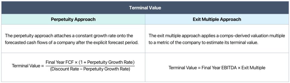
- The Growth in Perpetuity Approach assumes a constant growth rate for cash flows beyond the forecast period, while the Exit Multiple Approach applies a valuation multiple to a financial metric, such as EBITDA, to estimate terminal value: Terminal Value = Final Year EBITDA × Exit Multiple
- The formula to calculate the terminal value using the growth in perpetuity approach involves the following formula: Terminal Value = (Final Year FCF × (1 + Perpetuity Growth Rate)) ÷ (Discount Rate – Perpetuity Growth Rate).
- The terminal value must be discounted to the current date using the following formula: Present Value of Terminal Value = Terminal Value ÷ (1 + Discount Rate)^Number of Years.
How to Calculate Terminal Value (TV)
The terminal value (TV) is the estimated value of a company beyond the initial forecast period in a DCF model.
The premise of the DCF approach states that an asset (i.e., the company) is worth the sum of all of its future free cash flows (FCFs), which must discounted to the present day.
Projected cash flows must be discounted to their present value (PV) because a dollar received today is worth more than dollar received on a later date (i.e. the fundamental “time value of money” concept).
Since it is not feasible to project a company’s FCF indefinitely, the standard structure used most often in practice is the two-stage DCF model.
- Explicit FCF Forecast (~5-10 years)
- Terminal Value (TV)
The accuracy of forecasting tends to reduce in reliability the further out the projection model tries to predict operating performance.
On that note, simplified high-level assumptions eventually become necessary to capture the lump sum value at the end of the forecast period, or “terminal value”.
In practice, there are two widely used methods to calculate the terminal value as part of performing a DCF analysis.
- Growth in Perpetuity Approach
- Exit Multiple Approach
Terminal Value Formula: Growth in Perpetuity Approach
The growth in perpetuity approach assigns a constant growth rate to the forecasted cash flows of a company after the explicit forecast period.
Under the perpetuity growth method, the terminal value is calculated by treating a company’s terminal year free cash flow (FCF) as a growing perpetuity at a fixed rate.
The formula under the perpetuity approach involves taking the final year’s FCF and growing it by the long-term growth rate assumption and then dividing that amount by the discount rate minus the perpetuity growth rate.
Here, the terminal value is reliant on two major assumptions:
- Discount Rate (r)
- Perpetuity Growth Rate (g)
If the cash flows being projected are unlevered free cash flows, then the proper discount rate to use would be the weighted average cost of capital (WACC) and the ending output is going to be the enterprise value.
But if the cash flows are levered FCFs, the discount rate should be the cost of equity and the equity value is the resulting output.
One of the first steps to building a DCF is projecting the company’s future FCFs until its financial performance has reached a normalized “steady state”, which subsequently serves as the basis for the terminal value under the growth in perpetuity approach.
The long-term growth rate should theoretically be the growth rate that the company can sustain into perpetuity. Often, GDP growth or the risk-free rate can serve as proxies for the growth rate.
Given how terminal value (TV) accounts for a substantial portion of a company’s valuation, cyclicality or seasonality patterns must not distort the terminal year.
The long-term growth rate assumption should generally range between 2% to 4% to reflect a realistic, sustainable rate.
Otherwise, the implicit assumption of an excessively high growth rate (i.e., >5%) is that the company is on track to someday outpace the growth of the global economy – which is an unrealistic scenario, at the risk of stating the obvious.
Closely tied to the revenue growth, the reinvestment needs of the company must have also normalized near this time, which can be signified by:
- Depreciation converges toward equaling Capex (i.e. near 100% ratio)
- Capex as a percentage of revenue ranges near the lower end of what is typical in the company’s industry (i.e., the majority of Capex is now maintenance-related)
One frequent mistake is cutting off the explicit forecast period too soon, when the company’s cash flows have yet to reach maturity.
How to Calculate Present Value of Terminal Value (PV)
A perpetuity is defined as a security (e.g., bond) with no fixed maturity date, and the formula for calculating the present value (PV) is the cash flow value divided by the discount rate (i.e., the expected rate of return based on the risks associated with receiving the cash flows).
For instance, if the cash flow at the end of the initial forecast period is $100 and the discount rate is 10.0%, the TV comes out to $1,000 ($100 ÷ 10.0%).
But as mentioned earlier, the perpetuity growth method assumes that a company’s cash flows grow at a constant rate perpetually.
Because of this distinction, the perpetuity formula must account for the fact that there is going to be growth in cash flows, as well. Hence, the denominator deducts the growth rate from the discount rate.
If the cash flow at the end of the initial projection period is $100 and the discount rate is 10.0% but this time around, there is a perpetuity growth rate of 3%, the terminal value comes out as ~$1,471.
- Terminal Value = ([$100 x (1 + 3.0%)] ÷ [10.0% – 3.0%]) = ~$1,471
Terminal Value Formula: Exit Multiple Approach
The exit multiple approach applies a valuation multiple to a metric of the company to estimate its terminal value.
In theory, the exit multiple serves as a useful point of reference for the future valuation of the target company in its mature state.
The formula for the TV using the exit multiple approach multiplies the value of a certain financial metric (e.g., EBITDA) in the final year of the explicit forecast period by an exit multiple assumption.
The exit multiple assumption is derived from market data on the current public trading multiples of comparable companies and multiples obtained from precedent transactions of comparable targets.
The exit multiple method also comes with its share of criticism as its inclusion brings an element of relative valuation into intrinsic valuation.
The DCF model utilizes a fundamentals-oriented perspective and one of the touted benefits is its independence from prevailing market valuations, which can be prone to mispricing at times due to irrational investor sentiment (e.g., short-term overreactions).
But compared to the perpetuity growth approach, the exit multiple approach tends to be viewed more favorably because the assumptions used to calculate the TV can be better explained (and are thus more defensible).
The growth rate in the perpetuity approach can be seen as a less rigorous, “quick and dirty” approximation – even if the values under both methods differ marginally.
In either approach, TV represents the present value of the company’s cash flows in the final year of the explicit forecast period before entering the perpetuity stage (i.e. if Year 10 cash flows are used for the calculations, the resulting TV derived from the methods above represent the present value of the TV in Year 10).
Since the DCF is based on what a company is worth as of today, it is necessary to discount the future TV back to the present date (i.e. in the aforementioned example, the Year 10 TV needs to be discounted back to the equivalent Year 0 TV).
DCF Terminal Value Implied Growth Rate Formula
The perpetuity growth approach is recommended to be used in conjunction with the exit multiple approach to cross-check the implied exit multiple – and vice versa, as each serves as a “sanity check” on the other.
Unless there are atypical circumstances such as time constraints or the absence of data surrounding the valuation, the calculation under both methods is normally listed side-by-side.
For example, if the implied perpetuity growth rate based on the exit multiple approach seems excessively low or high, it may be an indication that the assumptions might require adjusting.
If the exit multiple approach was used to calculate the TV, it is important to cross-check the amount by backing into an implied growth rate to confirm that it’s reasonable.
In effect, the terminal value (TV) under either approach should be reasonably close – albeit, the exit multiple approach is viewed more favorably in practice due to the relative ease of justifying the assumptions used, especially since the DCF method is intended to be an intrinsic, cash-flow oriented valuation.
Terminal Value Calculator — Excel Template
We’ll now move to a modeling exercise, which you can access by filling out the form below.
1. DCF Model Assumptions
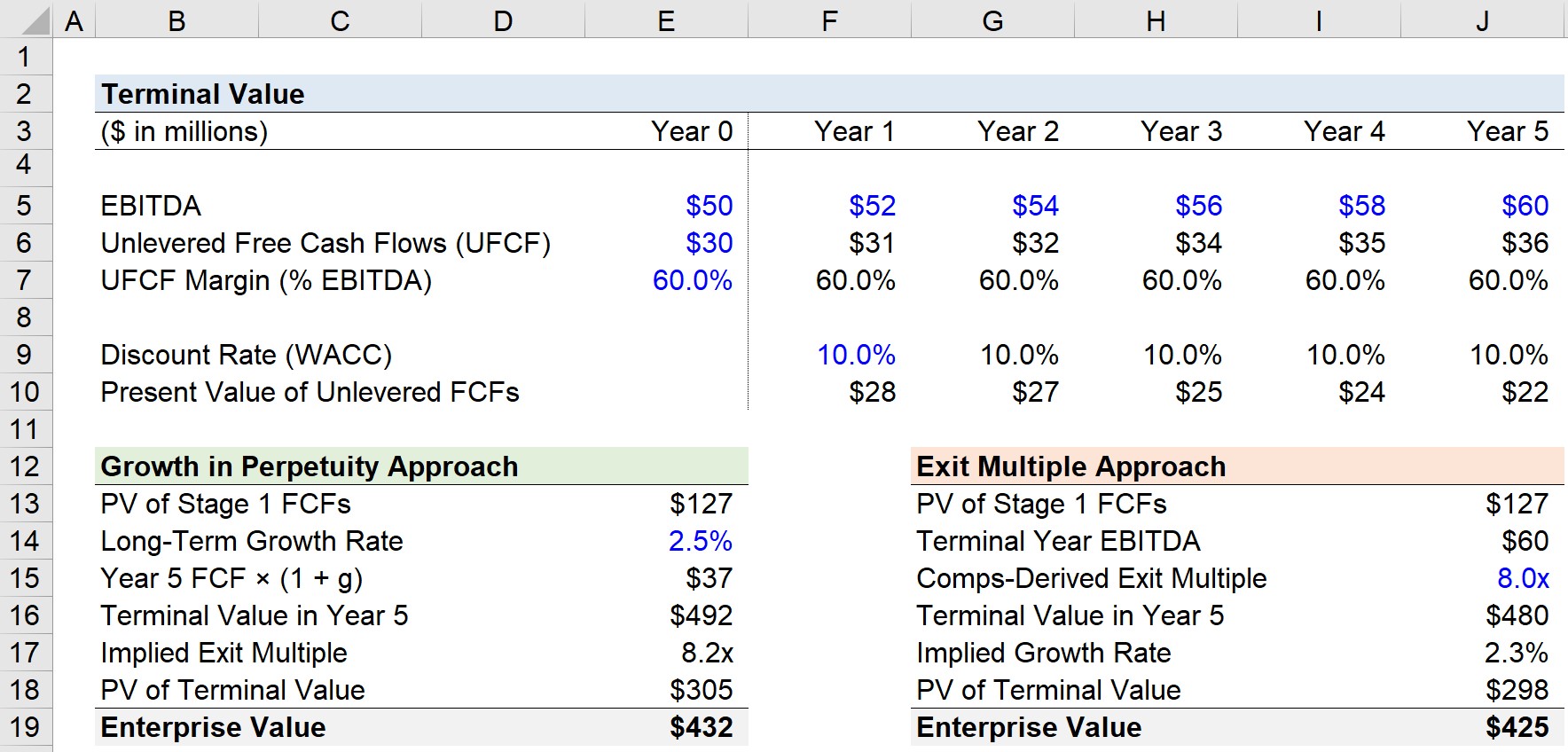
Let’s get started with the projected figures for our hypothetical company’s EBITDA and free cash flow. In the last twelve months (LTM), EBITDA was $50mm and unlevered free cash flow was $30mm.
From Year 1 to Year 5 – the forecasted range of stage 1 cash flows – EBITDA grows by $2mm each year and the 60% FCF to EBITDA ratio is assumed to remain fixed.
- FCF to EBITDA Ratio (%) = $30mm ÷ $50mm = 60%
The 60% FCF to EBITDA ratio assumption is extrapolated for each forecasted period.
For example, the FCF in “Year 5” is $36mm, which is computed by multiplying the $60mm in EBITDA by the 60.0% FCF conversion assumption.
In the next step, we’ll be summing up the PV of the projected cash flows over the next five years – i.e., how much all of the forecasted cash flows are worth today.
Since the discount rate assumption is hardcoded as 10.0%, we can divide each free cash flow amount by (1 + the discount rate), raised to the power of the period number.
For purposes of simplicity, the mid-year convention is not used, so the cash flows are being discounted as if they are being received at the end of each period.
Note the appropriate cash flows to select in the range should only consist of future cash flows and exclude any historical cash flows (e.g., Year 0).
Once we discount each FCF and sum up the values, we get $127mm as the PV of the stage 1 FCFs – and this amount remains constant under either approach.
2. Growth in Perpetuity Terminal Value Calculation
Now that we’ve finished projecting the stage 1 FCFs, we can move on to calculating the terminal value under the growth in perpetuity approach.
To be conservative, we’ll be using 2.5% as the long-term growth rate assumption.
Next, the Year 5 FCF of $36mm is going to be multiplied by the 2.5% growth rate to arrive at $37mm for the FCF value in the next year, which will then be inserted into the formula for the calculation.
Upon dividing the $37mm by the denominator consisting of the discount rate of 10% minus the 2.5%, we get $492mm as the terminal value (TV) in Year 5.
However, the calculated terminal value (TV) is as of Year 5, while the DCF valuation is based on the value on the present date.
Therefore, we must discount the value back to the present date to get $305mm as the PV of the terminal value (TV).
If we add the two values – the $127mm PV of stage 1 FCFs and $305mm PV of the TV – we get $432mm as the implied total enterprise value (TEV).
- Total Enterprise Value (TEV) = $127 million + $305 million = $432 million
3. Exit Multiple Terminal Value Calculation
Moving onto the other calculation method, we’ll now walk through the exit multiple approach.
The $127mm in PV of stage 1 FCFs was previously calculated and can just be linked to the matching cell on the left. Then, we’ll grab the terminal year EBITDA, which is $60mm in Year 5.
The exit multiple assumption we’ll use here is going to be 8.0x. By multiplying the $60mm in terminal year EBITDA by the comps-derived exit multiple assumption of 8.0x, we get $480mm as the TV in Year 5.
But once again, the PV of this amount must be calculated by dividing $480mm by (1 + 10% discount rate) raised to the power of 5, which comes out to $298mm.
The $425mm total enterprise value (TEV) was calculated by taking the sum of the $127mm present value (PV) of stage 1 FCFs and the $298mm in the PV of the terminal value (TV).
- Total Enterprise Value (TEV) = $127 million + $298 million = $425 million
4. DCF Terminal Value Example
In our final section, we’ll perform “sanity checks” on our calculations to determine whether our assumptions were reasonable or not.
Starting with the growth in perpetuity approach, we can back out the implied exit multiple by dividing the TV in Year 5 ($492mm) by the final year EBITDA ($60mm), which comes out to an implied exit multiple of 8.2x.
In the subsequent step, we can now figure out the implied perpetual growth rate under the exit multiple approach.
Considering the implied multiple from our perpetuity approach calculation based on a 2.5% long-term growth rate was 8.2x, the exit multiple assumption should be around that range.
The exit multiple used was 8.0x, which comes out to an implied terminal growth rate of 2.3% – a reasonable constant growth rate that confirms that our terminal value assumptions pass the “sanity check”.

Everything You Need To Master Financial Modeling
Enroll in The Premium Package: Learn Financial Statement Modeling, DCF, M&A, LBO and Comps. The same training program used at top investment banks.
Enroll Today


")