- What is Leverage Ratio?
- How to Calculate Leverage Ratio
- What are Balance Sheet Leverage Ratios?
- Leverage Ratio Calculation Example
- What are Cash Flow Leverage Ratios?
- Leverage Ratio Formula
- Credit Risk vs. Default Risk: What is the Difference?
- Leverage Ratio vs. Coverage Ratio: What is the Difference?
- What is the Role of Leverage Ratios in Loan Covenants?
- Leverage Ratio Calculator — Excel Calculator
- 1. Income Statement Assumptions
- 2. Leverage Ratio Calculation Example (Upside Case)
- 3. Leverage Ratio Analysis Example (Downside Case)
What is Leverage Ratio?
Leverage Ratio measures a company’s inherent financial risk by quantifying the reliance on debt to fund operations and asset purchases, whether it be via debt or equity capital.
The debt burden on the balance sheet of the borrower is compared to metrics that pertain to cash flow, assets, and total capitalization, which collectively help gauge the company’s credit risk (or risk of default).
- The leverage ratio quantifies a company's financial risk by measuring its reliance on debt for funding operations and asset acquisitions, helping to analyze credit risk and the potential for default.
- Leverage ratios can be calculated using various formulas, such as the debt-to-equity (D/E) and debt-to-assets ratios, which provide insights into the appropriate proportion of debt relative to equity and total assets, respectively.
- While debt can be a cost-effective financing source due to tax-deductible interest expenses, excessive reliance on debt increases financial risk, potentially leading to earnings volatility and default if cash flows are insufficient to meet obligations.
- Leverage ratios are critical in loan covenants, where lenders set maximum limits to control risk.
- Breaching a loan covenant can result in penalties or trigger an immediate repayment, illustrating the importance of maintaining sustainable debt levels.
How to Calculate Leverage Ratio
Companies require capital to operate and continue to deliver their products and services to their customers.
For a certain period, the cash generated by the company and the equity capital contributed by the founder(s) and outside equity investors could be enough.
However, for companies attempting to reach the next stage of growth by pursuing more ambitious plans for expansion, obtaining more market share, expanding their geographical reach, and engaging in M&A, debt financing can often become a necessity.
The standard composition of a company’s capital structure consists of:
- Common Stock ➝ The most basic level of corporate ownership that typically comes with voting rights – i.e. the lowest priority ownership claim in a company.
- Preferred Stock ➝ Considered a hybrid between common stock and debt instruments, blending properties of each – for example, preferred shares hold priority claim over common shareholders yet have no voting rights and receive fixed dividend payments similar to interest expense payments.
- Total Debt ➝ Capital borrowed from lenders with the company acting as a borrower – which is agreed upon in exchange for scheduled interest expense payments throughout the term of the debt as well as the full repayment of the original principal amount on the date of maturity.
Of the various benefits of using debt capital, one notable advantage is related to interest expense being tax-deductible (i.e. the “tax shield”), which lowers the taxable income of a company and the amount in taxes paid.
Considering how debt is placed higher in the capital structure and receives priority treatment over both preferred and common shareholders, the cost of debt tends to be lower relative to the cost of equity, which is placed at the very bottom of the capital structure.
However, debt financing comes with significant risks, and any company must be aware of the potential consequences of leverage, namely the increased volatility in earnings (i.e. EPS) and the potential for defaulting on debt obligations.
The reliance on leverage is neither inherently good nor bad. Instead, the issue is “excess” debt, in which the debt burden is unmanageable given the borrower’s free cash flow (FCF).
In fact, debt can be a “cheaper” source of financing compared to equity, and the interest tax shield can be beneficial for companies.
However, if the capital structure is unsustainable (i.e. overreliance on debt), the negative effects of debt financing soon become apparent.
What are Balance Sheet Leverage Ratios?
On the balance sheet, leverage ratios measure the financial leverage on the balance sheet of the company, or the reliance a company has on creditors to fund its operations.
Simply put, the concept of financial leverage refers to the proportion of debt in the capital structure, rather than equity.
The questions answered here are, “What is the current mixture of debt and equity in the company’s capital structure?” and “Is the current debt-to-equity (D/E) ratio sustainable?”
For a company dependent on creditors (e.g. to purchase inventory or fund capital expenditures), the unexpected cut-off in access to external financing could be detrimental to its ability to continue operating as a “going concern.”
- High Financial Leverage ➝ Significant reliance on external debt financing sources
- Low Financial Leverage ➝ Operations are funded mostly with internally generated cash (i.e. retained earnings)
In general, increased amounts of leverage in the capital structure equates to more financial risk, since the company incurs greater interest expense and mandatory debt amortization as well as principal repayments coming up in the future.
But if a company opts to use very minimal leverage, the downside is that there are more shareholders with claims to the same amount of net profits, which results in fewer returns for all equity holders – all else being equal.
Not to mention, the company is unable to benefit from the reduced taxes associated with the tax-deductibility of interest expense or the lower cost of capital (i.e. debt is a cheaper source of capital than equity up to a certain point).
| Leverage Ratio Type | Purpose | Formula |
| Debt-to-Assets Ratio (D/A) |
|
|
| Debt-to-Equity Ratio (D/E) |
|
|
| Debt-to-Total Capitalization |
|
|
|
Net Debt-to-Total Capitalization
|
|
|
Leverage Ratio Calculation Example
Suppose there’s a company with the following balance sheet data:
- Total Assets = $70 million
- Total Debt = $30 million
- Total Equity = $40 million
To calculate the B/S ratios, we’d use the following formulas:
- Debt-to-Equity = $30 million ÷ $40 million = 0.8x
- Debt-to-Assets = $30 million ÷ $70 million = 0.4x
- Debt-to-Total Capitalization = $30 million ÷ ($30 million + $40 million) = 0.4x
What are Cash Flow Leverage Ratios?
An alternative approach is to measure financial risk using cash flow leverage ratios, which help determine if a company’s debt burden is manageable given its fundamentals (i.e. ability to generate cash).
In practice, these types of ratios measure the proportion of a company’s debt amount to another financing metric (e.g. equity, asset, total capitalization) or to a cash-flow metric to see if the company’s FCF generation could support payments on debt, most notably:
- Interest Expense Payments
- Required Debt Amortization
- Full Principal Repayments on Date of Maturity
The more predictable the cash flows of the company and consistent its historical profitability has been, the greater its debt capacity and tolerance for a higher debt-to-equity (D/E) mix.
The cash flow variation is arguably a more practical approach in thinking about the financial risk of a company since you’re comparing two off-setting factors:
- “How much does the company owe?”
- “How much cash flow does the company generate?”
The purpose is to assess if the company’s cash flows can adequately handle existing debt obligations.
If yes, the company’s debt-related payments, such as interest expense and principal repayment, are supported by its cash flows, and payments can be met on schedule.
Lenders and credit analysts most commonly use the total debt-to-EBITDA ratio, but there are numerous other variations.
| Ratio Type | Description | Formula |
| Total Debt-to-EBITDA |
|
|
| Net Debt-to-EBITDA |
|
|
| Total Debt-to-EBIT |
|
|
| Total Debt-to-EBITDA Less Capex |
|
|
Each of these measures, regardless of the cash flow metric chosen, shows the number of years of operating earnings that would be required to clear out all existing debt.
In effect, leverage ratios provide more insights into the ability of the company’s cash flows to cover upcoming debt obligations, as opposed to a proportion of how levered a particular company’s capital structure is.
Leverage Ratio Formula
Note that if you ever hear someone refer to the “leverage ratio” without any further context, it is safe to assume that they are talking about the debt-to-EBITDA ratio.
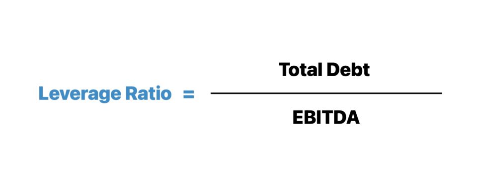
The leverage ratio—or debt-to-EBITDA ratio—is calculated by dividing the total debt balance by EBITDA in the coinciding period.
Here, EBITDA is used as a proxy for operating cash flow, and the question being answered is: “Is the company’s cash flow generation capacity enough to satisfy its outstanding financial obligations?”
EBITDA is the most widely used proxy for operating cash flow despite its shortcomings, such as ignoring the full cash impact of capital expenditures (CapEx).
For highly cyclical, capital-intensive industries in which EBITDA fluctuates significantly due to inconsistent CapEx spending patterns, using (EBITDA – CapEx) can be more appropriate.
The senior debt ratio is important to track because senior lenders are more likely to place covenants – albeit, such restrictions have loosened across the past decade (i.e. “covenant-lite” loans).
Many perceive the net debt ratio as a more accurate measure of financial risk since it accounts for the cash sitting on the borrower’s balance sheet (B/S), which reduces the risk to the lender(s).
Each of the acceptable ranges for the listed ratios is contingent on the industry and characteristics of the specific business, as well as the prevailing sentiment in the credit markets.
Credit Risk vs. Default Risk: What is the Difference?
The default risk is a sub-set of credit risk that refers to the risk that the borrower might default on (i.e. fail to repay) its debt obligations.
Excessive reliance on debt financing could lead to a potential default and eventual bankruptcy in the worst-case scenario.
Often, a company will raise debt capital when it is well-off financially, and operations appear stable, but downturns in the economy and unexpected events can quickly turn the company’s trajectory around.
Sometimes the best course of action could be to potentially hire a restructuring advisory firm in anticipation of a missed interest payment (i.e. default on debt) or breached loan covenant.
From a restructuring standpoint, the earlier the company can get in front of the problem without involving the Bankruptcy Court, the better off the company is likely going to be.
Leverage Ratio vs. Coverage Ratio: What is the Difference?
Leverage ratios set a ceiling on the debt levels of a company, whereas coverage ratios set a minimum floor that the company’s cash flow cannot fall below.
- Higher Leverage Ratio ➝ Higher leverage ratios typically indicate that the company has raised debt capital near its full debt capacity or beyond the amount it could reasonably handle.
- Lower Leverage Ratio ➝ Unlike coverage ratios, lower leverage ratios are viewed as positive signs of financial health.
For example, the higher the times interest earned ratio (TIE), the better off the company is from a risk perspective.
Why? A higher TIE ratio implies the company can pay off its interest expense multiple times using the cash flows it generates.
In contrast, higher leverage relative to comparable peers could be concerning, especially if the ratio has been trending upward in recent periods, as the two potential drivers are:
- EBITDA ➝ The proxy for operating cash flow, EBITDA, has been declining.
- Debt Balance ➝ The amount of total debt outstanding has remained constant (or potentially increased).
From the perspective of lenders, a higher ratio of debt relative to its cash flow, assets, or equity indicates the company chose to take on a large amount of debt, thereby increasing the likelihood that it could fail to service a debt payment on time due to lack of liquidity or cash flows.
What is the Role of Leverage Ratios in Loan Covenants?
In loan agreements and other lending documents, leverage ratios are one method for lenders to control risk and ensure the borrower does not take any high-risk action that places its capital at risk.
For instance, lenders could set maximum limits for total leverage metrics within their credit agreements.
If the borrower breaches the agreement and the ratio exceeds the agreed-upon ceiling, the contract could treat that as a technical default, resulting in a monetary fine and/or the immediate repayment of the full original principal.
In particular, senior lenders, such as corporate banks, tend to be more strict when negotiating lending terms regarding the requirements that the borrower must abide by.
There are two main types of debt covenants: maintenance and incurrence covenants.
- Maintenance Covenants ➝ Maintenance covenants are contractual agreements requiring the borrower to maintain compliance with certain credit metrics, with periodic testing performed at the end of each quarter. Often, the maintenance covenants are cash flow ratios, e.g. Total Debt-to-EBITDA cannot exceed 6.0x, and Senior Debt-to-EBITDA cannot exceed 3.0x.
- Incurrence Covenants ➝ Lenders often also place restrictions meant to impede certain actions, such as issuing dividends to shareholders or raising more debt beyond a certain level. For these so-called “incurrence” covenants, testing is done once “triggering events” occur to confirm that the borrower still complies with lending terms – e.g. issuing additional debt, debt-funded M&A, cash dividends to shareholders, share repurchases, etc.
Leverage Ratio Calculator — Excel Calculator
We’ll now move to a modeling exercise, which you can access by filling out the form below.
1. Income Statement Assumptions
In the first section of our modeling exercise, we’ll start by providing the model assumptions.
Here, we’ll be analyzing our company’s credit risk profile under two different operating scenarios:
- “Upside” Case
- “Downside” Case
For either case, the starting point will be 2021, from which we’ll be adding the balance to the step function for the applicable line items.
- Revenue: $125m
- EBITDA: 40% Margin → $50m
- EBIT: 30% Margin → $38m
Next, we’ll state the assumptions regarding the year-over-year (YoY) changes for both the “Downside” and the “Upside” cases.
Upside Case – Step Function
- Revenue % Growth: +1.0%
- EBITDA % Margin: +2.5%
- EBIT % Margin: +2.0%
Downside Case – Step Function
- Revenue % Growth: –2.0%
- EBITDA % Margin: –2.5%
- EBIT % Margin: –2.0%
As for the capitalization section, we only require two metrics:
- Cash & Equivalents: Cash and highly liquid assets (e.g. marketable securities)
- Total Debt: Both long-term and short-term debt, as well as any interest-bearing instruments
From those two metrics, we can calculate the net debt balance by subtracting the cash balance from the total debt outstanding.
In 2021, our company has $50m in “Cash & Equivalents” and $200m in “Total Debt”, which is comprised of $150m in “Senior Debt” and $50m in “Subordinated Debt”.
Upside Case – Step Function
- Cash & Equivalents: +$5m
- Senior Debt: –$10m
- Subordinated Debt: –$5m
Downside Case – Step Function
- Cash & Equivalents: –$10m
- Senior Debt: –$5m
- Subordinated Debt: –$2m
In the “Upside” case, the company is generating more revenue at higher margins, which results in greater cash retention on the balance sheet.
The increase in free cash flow (FCF) also means more discretionary debt can be paid down (i.e. optional prepayment), which is why the debt repayment is greater relative to the other case.
Conversely, in the “Downside Case, the company’s revenue is growing at a negative rate with lower margins, which causes the cash balance of the company to decline.
The debt repayment is lower in the second scenario, as only the mandatory amortization payments are made, as the company does not have the cash flow available for the optional paydown of debt.
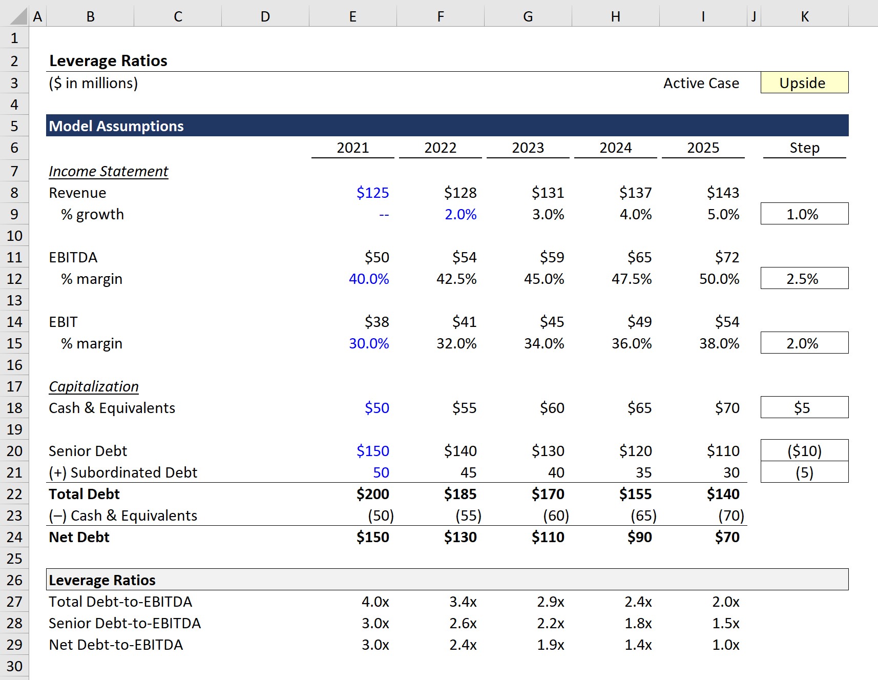
2. Leverage Ratio Calculation Example (Upside Case)
Now, we have all the required inputs for our model to calculate three important ratios using the following formulas.
- Total Debt-to-EBITDA = Total Debt ÷ EBITDA
- Senior Debt-to-EBITDA = Senior Debt ÷ EBITDA
- Net Debt-to-EBITDA = Net Debt ÷ EBITDA
Under the “Upside” case, our total debt-to-EBITDA declines in half from 4.0x to 2.0x from 2021 to 2025, which is attributable to the increased free cash flow (FCF) generation, higher profit margins, and greater cash balance.
The senior leverage variation is also reduced by half from 3.0x to 1.5x—which is caused by the increased discretionary paydown of the debt principal (i.e. –$10m each year).
In the same time horizon, the net debt variation falls from 3.0x to 1.0x, with the total accumulation of cash being the most significant contributor.
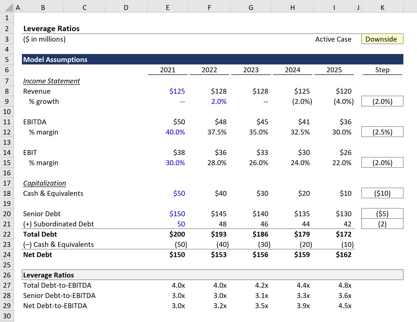
3. Leverage Ratio Analysis Example (Downside Case)
In the final section of our model exercise, we’ll perform the same calculations but under the “Downside” scenario.
As expected, each of the ratios increases as a result of the sub-par performance of the company.
From 2021 to the end of 2025, the total leverage ratio increased from 4.0x to 4.8x, the senior ratio increased from 3.0x to 3.6x, and the net debt ratio increased from 3.0x to 4.5x.
Because of the diminished cash balance, the net debt-to-EBITDA ratio is marginally lower than the total debt-to-EBITDA ratio by the end of Year 5.
In this case, the company’s senior lenders would likely become concerned regarding the borrower’s default risk since the senior ratio exceeds 3.0x, which is on the higher end of their typical lending parameters.

Everything You Need To Master Financial Modeling
Enroll in The Premium Package: Learn Financial Statement Modeling, DCF, M&A, LBO and Comps. The same training program used at top investment banks.
Enroll Today")
")