Basic LBO Modeling Test

Basic LBO Model Test: Practice Tutorial Guide

The following LBO model test is an appropriate place to start to ensure you understand the modeling mechanics, particularly for those starting to prepare for private equity interviews.

But for investment banking analysts interviewing for PE, expect more challenging LBO modeling tests like our Standard LBO modeling test or even an advanced LBO modeling test.

The format for the basic LBO model is as follows.

• Excel Usage: Unlike the paper LBO, which is a pen-and-paper exercise given in earlier stages of the PE recruiting process, in an LBO Modeling Test candidates are given access to Excel and expected to construct an operating and cash flow forecast, financing sources & uses and ultimately determine the implied investment returns and other key metrics based on the information provided in the prompt.
• Time Limit: The various LBO Excel modeling tests you encounter throughout the recruitment process will most commonly be either 30 minutes, 1 hour or 3 hours depending on the firm and how near you are to the final stage before offers are made. The one covered in this post should take approximately one hour at most, assuming that you’re starting from a blank spreadsheet.
• Prompt Format: In some cases, you will be provided a brief prompt consisting of a few paragraphs on a fictitious scenario and be asked to build a quick model from scratch – whereas in others, you may be given the confidential information memorandum (“CIM”) of a real acquisition opportunity to put together an investment memo alongside an LBO model to support your thesis. For the latter, the prompt is usually left vague intentionally and it will be asked in the form of a “share your thoughts” open-ended context.

LBO Model Interview Grading Criteria

Every firm has a slightly different grading rubric for the LBO modeling test, yet at its core, most boil down to two criteria:

1. Accuracy: How well do you understand the underlying mechanics of an LBO model?
2. Speed: How quickly can you complete the task without a loss in accuracy?

For more complex case studies, where you will be given more than three hours, your ability to interpret the output of the model and make an informed investment recommendation will be just as important as your model flowing correctly with the right linkages.

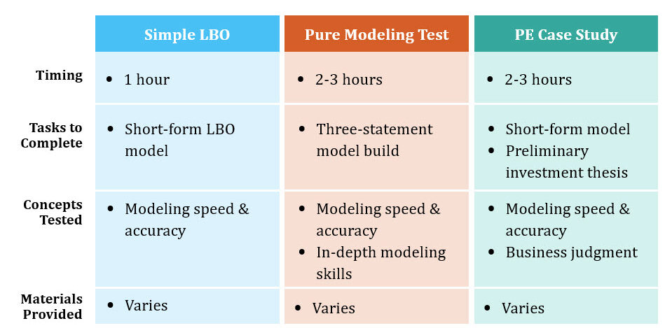
^{In-Person LBO Modeling Test Spectrum}

LBO Model Test Example: Illustrative Prompt

Let’s get started! An illustrative prompt on a hypothetical leveraged buyout (LBO) can be found below.

LBO Model Test Instructions

A private equity firm is considering the leveraged buyout of JoeCo, a privately-owned coffee company. In the last twelve months (“LTM”), JoeCo generated $1bn in revenue and $100mm in EBITDA. If acquired, the PE firm believes JoeCo’s revenue can continue to grow 10% YoY while its EBITDA margin remains constant.

To fund this transaction, the PE firm was able to obtain 4.0x EBITDA in Term Loan B (“TLB”) financing – which will come with a seven-year maturity, 5% mandatory amortization, and priced at LIBOR + 400 with a 2% floor. Packaged alongside the TLB is a $50mm revolving credit facility (“revolver”) priced at LIBOR + 400 with an unused commitment fee of 0.25%. For the last debt instrument used, the PE firm raised 2.0x in Senior Notes that carries a seven-year maturity and an 8.5% coupon rate. The financing fees were 2% for each tranche while the total transaction fees incurred were $10mm.

On JoeCo’s balance sheet, there is $200mm of existing debt and $25mm in cash, of which $20mm is considered excess cash. The business will be delivered to the buyer on a “cash-free, debt-free basis”, which means the seller is responsible for extinguishing the debt and keeps all the excess cash. The remaining $5mm in cash will come over in the sale, as this is cash that the parties determined is required to keep the business operating smoothly.

Assume for each year that JoeCo’s depreciation & amortization expense (“D&A”) will be 2% of revenue, capital expenditures (“Capex”) requirement will be 2% of revenue, the change in net working capital (“NWC”) will be 1% of revenue, and the tax rate will be 35%.

If the PE firm were to purchase JoeCo at 10.0x LTM EV/EBITDA on 12/31/2020 and then exit at the same LTM multiple after a five-year time horizon, what would the implied IRR and cash-on-cash return of the investment be?

LBO Model Test – Excel Template

Use the form below to download the Excel file used to complete the modeling test.

However, while most firms will provide the financials in an Excel format that you could use as a “guiding” template, you should still be comfortable with creating a model starting from scratch.

AMEX

First Name *

Email *

Submit

By submitting this form, you consent to receive email from Wall Street Prep and agree to our terms of use and privacy policy.

Email provided

Your Download is Ready

Submitting...

Step 1. Model Assumptions

Entry Valuation

The first step of the LBO modeling test is to determine the entry valuation of JoeCo on the date of initial purchase.

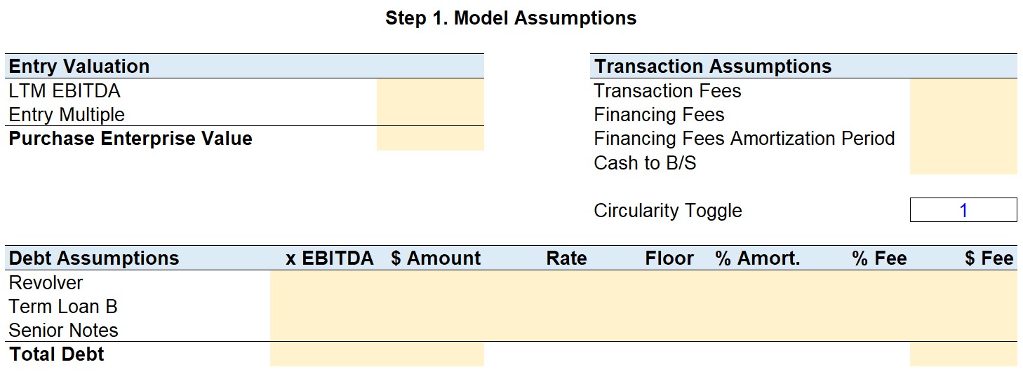
By multiplying JoeCo’s $100mm LTM EBITDA by the entry multiple of 10.0x, we know the enterprise value at purchase was $1bn.

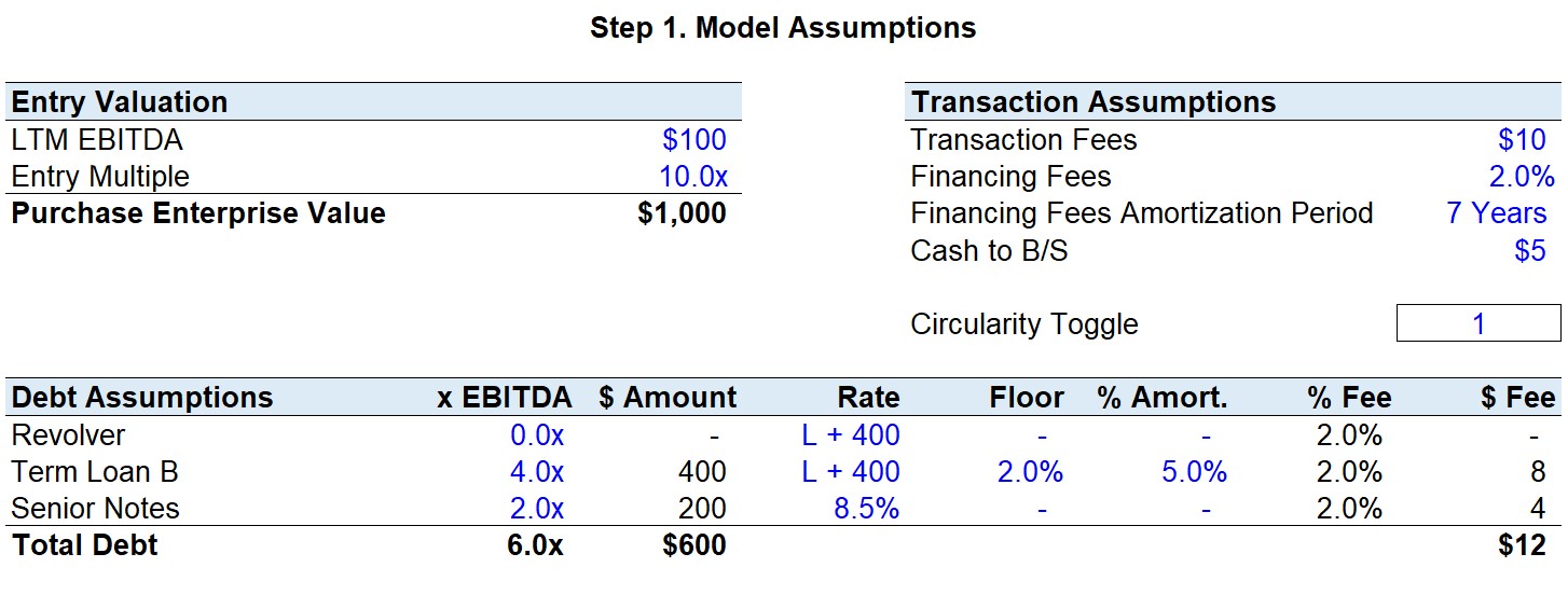
Transaction Assumptions

Next, we will list out the transaction assumptions provided.

• Transaction Fees: The transaction fees were $10mm – this is the amount paid to investment banks for their M&A advisory work, as well as to lawyers, accountants, and consultants that helped on the deal. These advisory fees are treated as a one-time expense, as opposed to being capitalized.
• Financing Fees: The 2% deferred financing fee refers to the costs incurred while raising debt capital to fund this transaction. This financing fee will be based on the total magnitude of debt used and will be amortized over the tenor (term) of the debt – which is seven years in this scenario.
• Cash to B/S: The minimum cash balance required post-closing of the transaction (i.e. “Cash to B/S”) was stated as $5mm, which means JoeCo needs $5mm in cash-on-hand to continue operating and meet its short-term working capital obligations.

Debt Assumptions

With the entry valuation and transaction assumptions filled out, we can now list out the debt assumptions related to each debt tranche, such as the turns of EBITDA (“x EBITDA”), pricing terms, and amortization requirements.

The amount of debt that a lender has provided is expressed as a multiple of EBITDA (also called a “turn”). For instance, we can see $400mm was raised in Term Loan B as the amount was 4.0x EBITDA.

In total, the initial leverage multiple used in this transaction was 6.0x – since 4.0x was raised from TLB and 2.0x in Senior Notes.

Moving onto the columns on the right, the “Rate” and “Floor” are used to calculate the interest rate of each debt tranche.

The two senior secured debt tranches, the Revolver and Term Loan B are priced off LIBOR + a spread (i.e. priced at a “floating rate“), meaning that the interest rate paid on these debt instruments fluctuates based on LIBOR (“London Interbank Offered Rate”), the global standard benchmark used to set lending rates.

The general convention is to state the pricing of debt in terms of basis points (“bps”) rather than by “%”. The “+ 400” just means 400 basis points, or 4%. Therefore, the interest rate pricing on the Revolver and TLB will be LIBOR + 4%.

The Term Loan B tranche has a 2% “Floor”, which reflects the minimum amount required to be added to the spread. LIBOR will often fall below the floor rate during periods of low interest rates, so this feature is meant to ensure that a minimum yield is received by the lender.

For example, if LIBOR was at 1.5% and the floor was 2.0%, the interest rate on this Term Loan B would be 2.0% + 4.0% = 6.0%. But if LIBOR was at 2.5%, the interest rate on the TLB would be 2.5% + 4% = 6.5%. As you can see, the interest rate cannot fall below 6% because of the floor.

The third tranche of debt used, the Senior Notes, is priced at 8.5% (i.e. priced at a “fixed rate”). This type of pricing is simpler because regardless of whether LIBOR goes up or down, the interest rate will remain unchanged at 8.5%.

In the final column, we can calculate the financing fees based on the amount of debt raised. Since $400mm was raised in Term Loan B and $200mm was raised in Senior Notes, we can multiply each by the 2% financing fee assumption and sum them up to arrive at $12mm in financing fees.

Step 1: Formulas Used

• Purchase Enterprise Value = LTM EBITDA × Entry Multiple
• Debt Amount (“$ Amount”) = Debt EBITDA Turns × LTM EBITDA
• Financing Fees (“$ Fee”) = Debt Amount × % Fee

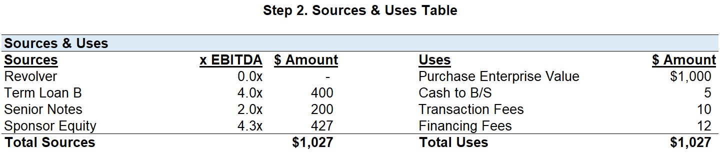
Step 2. Sources & Uses Table

In the next step, we will build out the Sources & Uses schedule, which lays out how much it will cost in total to acquire JoeCo and where the required funding will come from.

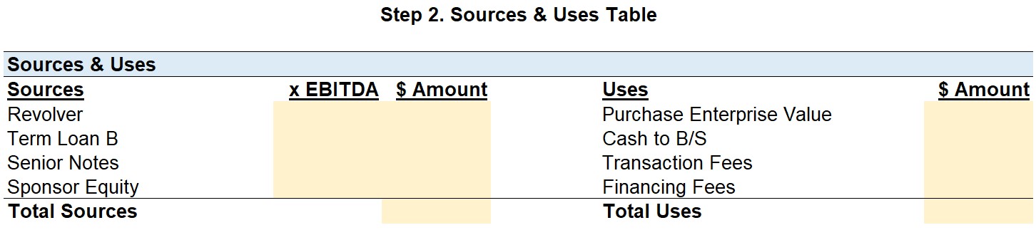
Uses Side

It is recommended to start on the “Uses” side and then complete the “Sources” side afterward since you need to figure out how much something costs before thinking about how you will come up with the funds to pay for it.

• Purchase Enterprise Value: To start, we have already calculated the “Purchase Enterprise Value” in the previous step and can directly link to it. The $1bn is the total amount being offered by the private equity firm to acquire the equity of JoeCo.
• Cash to B/S: We must recall that JoeCo’s cash balance cannot dip below $5mm post-transaction. As a result, the “Cash to B/S” in effect will increase the total funding required – hence, it will be on the “Uses” side of the table.
• Transaction Fees and Financing Fees: To finish the Uses section, the $10mm in transaction fees and $12mm in financing fees were already calculated earlier and can be linked to the relevant cells.

Therefore, $1,027mm in total capital will be required to complete this proposed acquisition of JoeCo, and the “Sources” side will now illustrate how the PE firm intends to finance the acquisition.

Sources Side

We will now outline how the PE firm came up with the necessary funds to meet the cost of purchasing JoeCo.

• Revolver: Since there was no mention of the revolving credit line being drawn, we can assume that none was used to help fund the purchase. The revolver is generally undrawn at close but could be drawn from if needed. Think of the revolver as a “corporate credit card” meant for use during emergencies – this line of credit is extended to borrowers by lenders to make their financing packages more attractive (i.e. for the Term Loan B in this scenario) and to provide JoeCo a “cushion” for unexpected liquidity shortages.
• Term Loan B (“TLB”): Next, a term loan B is provided by an institutional lender and is generally a senior, 1st lien loan with a 5 to 7 year maturity and low amortization requirements. The amount of TLB raised was calculated earlier by multiplying the 4.0x TLB leverage multiple by the LTM EBITDA of $100mm – thus, $400mm in TLB was raised to fund this purchase.
• Senior Notes: The third debt tranche raised was Senior Notes at a leverage multiple of 2.0x EBITDA, so $200mm was raised. Senior Notes are junior to secured bank debt (e.g. Revolver, Term Loans), and provide a higher yield to compensate the lender for undertaking the additional risk of holding a debt instrument lower in the capital structure.

Now that we have determined how much the firm needs to pay and the amount of debt funding, the “Sponsor Equity” is the plug for the remaining funds needed.

If we add up all the funding sources (i.e. the $600mm raised in debt) and then deduct it from the $1,027mm in “Total Uses”, we see $427mm was the initial equity contribution by the sponsor.

Step 2: Formulas Used

• Sponsor Equity = Total Uses – (Revolver + Term Loan B + Senior Notes Amounts)
• Total Sources = Revolver + Term Loan B + Senior Notes + Sponsor Equity

Step 3. Free Cash Flow Projection

Revenue and EBITDA

Thus far, the Sources & Uses table has been completed and the transaction structure has been determined, meaning that the free cash flows (“FCFs”) of JoeCo can be projected.

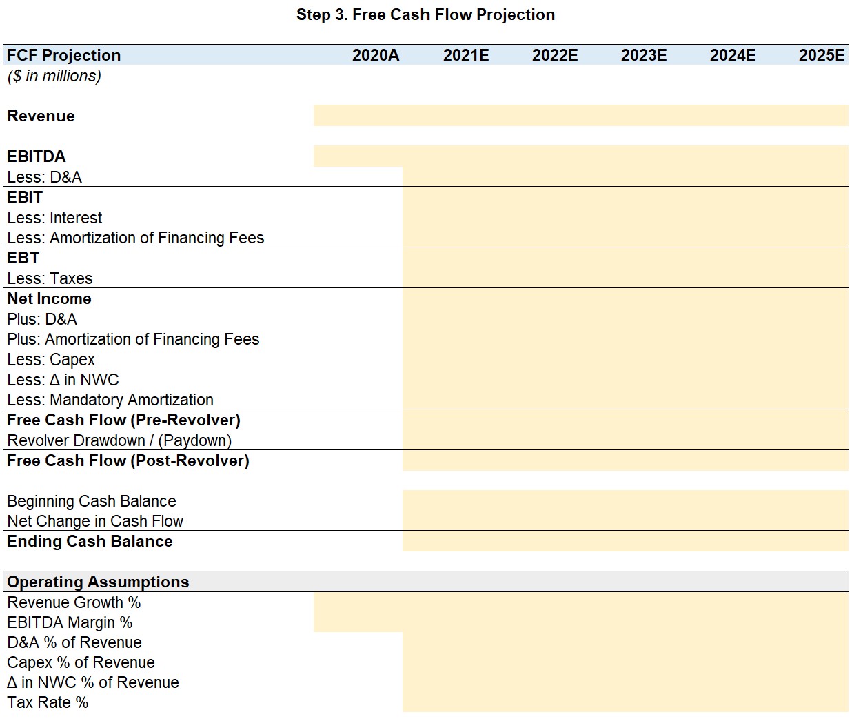
To start the forecast, we begin with Revenue and EBITDA since most of the operating assumptions provided are driven by a certain percentage of revenue.

As a general modeling best practice, it is recommended to place all the drivers (i.e. operating assumptions”) grouped together in the same section near the bottom.

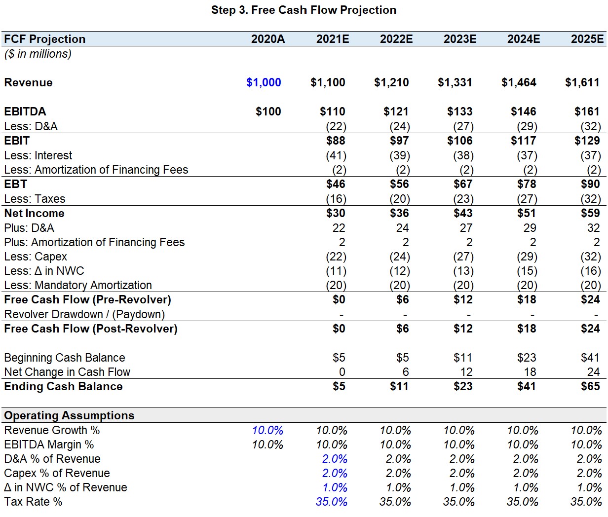
The prompt stated the year-over-year (“YoY”) revenue growth will be 10% throughout the holding period with the EBITDA margins held constant from the LTM performance.

While the EBITDA margin was not explicitly stated in the prompt, we can divide the LTM EBITDA of $100mm by the $1bn in LTM revenue to get a 10% EBITDA margin.

Once you have inputted the revenue growth rate and EBITDA margin assumptions, we can project the amounts for the forecast period based on the formulas below.

Operating Assumptions

As stated in the prompt, D&A will be 2% of revenue, Capex requirements are 2% of revenue, the change in NWC will be 1% of revenue, and the tax rate will be 35%.

All these assumptions will remain unchanged throughout the forecast period; therefore, we can “straight-line” them, i.e. reference the current cell to the one on the left.

Net Income

The formula for free cash flow before any revolver drawdown / (paydown) begins with net income.

Therefore, we need to work our way down from EBITDA to net income (“the bottom line”), meaning the subsequent step is to subtract D&A from EBITDA to calculate EBIT.

We are now at Operating Income (EBIT) and will subtract “Interest” and the “Amortization of Financing Fees”.

The interest expense line item will remain blank for now as the debt schedule has not yet been completed – we will return to this later.

For the financing fees amortization, we can compute this by dividing the total financing fee ($12mm) by the tenor of the debt, 7 years – doing so will leave us with ~$2mm each year.

The only expenses remaining from Pre-Tax Income (EBT) are the taxes paid to the government. This tax expense will be based on JoeCo’s taxable income, therefore we will multiply the 35% tax rate by EBT.

Once we have the amount in taxes due each year, we will subtract that amount from EBT to arrive at net income.

Free Cash Flow (Pre-Revolver)

The FCFs generated are central to an LBO as they determine the amount of cash available for debt amortization and the servicing of the due interest expense payments each year.

To calculate the FCF, we will first add back D&A and the Amortization of Financing Fees to Net Income since they are both non-cash expenses.

We calculated them both earlier and can just link to them but with the signs flipped since we are adding them back (i.e. more cash than net income showed).

Next, we subtract out Capex and the change in NWC. An increase in Capex and NWC are both outflows of cash and decrease the FCF of JoeCo, thus make sure to insert a negative sign at the front of the formula to reflect this.

In the final step before arriving at FCF, we will deduct the mandatory debt amortization associated with the Term Loan B.

For the time being, we’ll keep this part blank and return it once the debt schedule has been finalized.

Step 3: Formulas Used

• Total Uses = Purchase Enterprise Value + Cash to B/S + Transaction Fees + Financing Fees
• Revenue = Prior Revenue × (1 + Revenue Growth %)
• EBITDA = Revenue × EBITDA Margin %
• Free Cash Flow (Pre-Revolver) = Net Income + Depreciation & Amortization + Mandatory Amortization
• Financing Fees – Capex – Change in Net Working Capital – Mandatory Amortization
• D&A = D&A % of Revenue × Revenue
• EBIT = EBITDA – D&A
• Amortization of Financing Fees = Financing Fees Amount ÷ Financing Fees Amortization Period
• EBT (aka Pre-Tax Income) = EBIT – Interest – Amortization of Financing Fees
• Taxes = Tax Rate % × EBT
• Net Income = EBT – Taxes
• Capex = Capex % of Revenue × Revenue
• Δ in NWC = (Δ in NWC % of Revenue) × Revenue
• Free Cash Flow (Pre-Revolver) = Net Income + D&A + Amortization of Financing Fees – Capex – Δ in NWC –  Mandatory Debt Amortization

If a line item has “Less” at the front, confirm it is reflected as a negative outflow of cash, and vice versa if it has “Plus” in front. Assuming you followed the sign conventions as recommended, you can just sum up net income with the five other line items to arrive at the pre-revolver FCF.

Step 4. Debt Schedule

The debt schedule is arguably the trickiest part of the LBO Modeling Test.

In the previous step, we calculated the free cash flow available before any revolver drawdown / (paydown).

The missing line items that we had skipped over earlier will be derived from the debt schedule to complete those FCF projections.

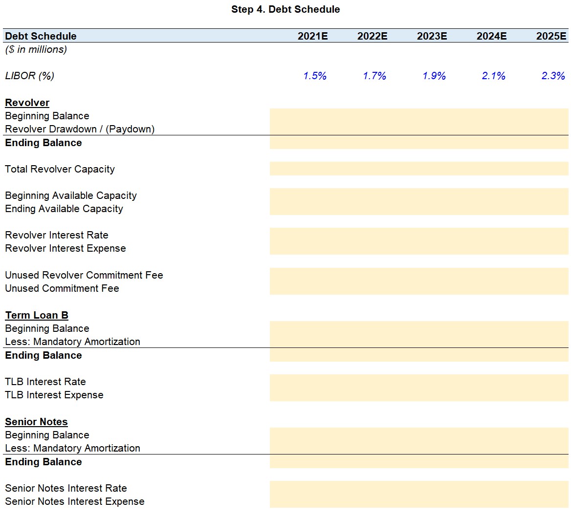
To take a step back, the purpose of creating this debt schedule is to keep track of JoeCo’s mandatory payments to its lenders and assess its revolver needs, as well as calculate the interest due from each debt tranche.

The borrower, JoeCo, is legally required to pay down debt tranches in a specific order (i.e. waterfall logic) and must abide by this lender agreement. Based on this contractual obligation, the revolver will be paid off first, followed by the Term Loan B, and then the Senior Notes.

The Revolver and TLBs are the highest in the capital structure and have the highest priority in the case of bankruptcy, hence carry a lower interest rate and represent “cheaper” sources of financing.

For each debt tranche, we will utilize roll-forward calculations, which refer to a forecasting approach that connects the current period forecast to the prior period after accounting for the line items that increase or decrease the ending balance.

Revolving Credit Facility (“Revolver”)

As mentioned in the beginning, the revolver functions similarly to a corporate credit card and JoeCo will draw down from it when it is short on cash and will pay off the balance once it has cash in excess.

If there is a shortage of cash, the revolver balance will rise – this balance will be paid down once there is a surplus of cash

The revolver sits at the very top of the debt waterfall and has the highest claim on JoeCo’s assets if the company were to be liquidated.

To start, we will create three line items:

1. Total Revolver Capacity
   The “Total Revolver Capacity” refers to the maximum amount that can be drawn from the revolver, and it comes out to $50mm in this scenario.
2. Beginning Available Revolver Capacity
   The “Beginning Available Revolver Capacity” is the amount that can be borrowed in the current period after deducting the amount already drawn in previous periods. This line item is calculated as the total revolver capacity minus the beginning of period balance.
3. Ending Available Revolver Capacity
   The “Ending Available Revolver Capacity” is the amount of the beginning available revolver capacity minus the amount drawn from in the current period.

For example, if JoeCo has drawn $10mm to date, the beginning available revolver capacity for the current period is $40mm.

To continue building out this revolver roll-forward, we link the beginning of period balance in 2021 to the amount of revolver used to fund the transaction in the Sources & Uses table. In this case, the revolver was left undrawn, and the beginning balance is thereby zero.

Then, the line that comes after will be “Revolver Drawdown / (Paydown)”.

The formula for the “Revolver Drawdown / (Paydown)” in Excel is shown below:

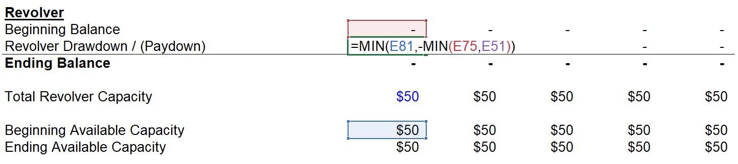
The “Revolver Drawdown” comes into play when the FCF of JoeCo has turned negative and the revolver will be drawn from.

Again, JoeCo can borrow at most up to the Available Revolver Capacity. This is the purpose of the 1st “MIN” function, it ensures no more than $50mm could be borrowed. It is entered as a positive because when JoeCo draws from the revolver, it is an inflow of cash.

The 2nd “MIN” function will return the lesser value between the “Beginning Balance” and the “Free Cash Flow (Pre-Revolver)”.

Take notice of the negative sign in front – in the case that the “Beginning Balance” is the smaller value of the two, the output will be negative and the existing revolver balance will be paid down.

The “Beginning Balance” figure cannot turn negative as that would imply that JoeCo paid down more of the revolver balance than it had borrowed (i.e. the lowest it can be is zero).

On the other hand, if the “Free Cash Flow (Pre-Revolver)” is the lesser value of the two, the revolver will be drawn from (as the two negatives will make a positive).

For instance, let’s say that JoeCo’s FCF has turned negative $5mm in 2021, the 2nd “MIN” function will output the negative free cash flow amount, and the negative sign placed in front will make the amount positive – which makes sense since this is a drawdown.

This is how the revolver balance would change if JoeCo’s pre-revolver FCF had turned negative by $5mm in 2021:

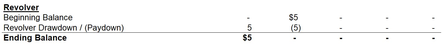
As you can see, the drawdown in 2021 would be $5mm. The ending balance of the revolver has increased to $5mm. In the next period, since JoeCo has sufficient pre-revolver FCF, it will pay down the outstanding revolver balance. The ending balance in the 2nd period has thus returned to zero.

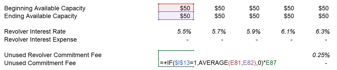
To calculate the interest expense associated with the revolver, we first need to get the interest rate. The interest rate is calculated as LIBOR plus the spread, “+ 400”. Since it was stated in terms of basis points, we divide 400 by 10,000 to get .04, or 4%.

Although the Revolver has no floor, it is a good habit to put the LIBOR rate in a “MAX” function with the floor, which is 0.0% in this case. The “MAX” function will output the larger value of the two, which is LIBOR in all the forecasted years. For example, the interest rate in 2021 is 1.5% + 4% = 5.5%.

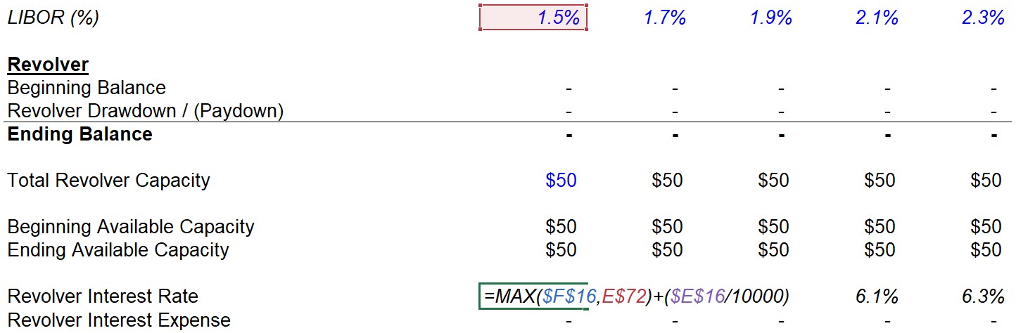
Note that if LIBOR were stated in basis points, the top line would look like “150, 170, 190, 210, and 230”. The formula would change in that LIBOR (Cell “F$73” in this case) will be divided by 10,000.

Now that we have calculated the interest rate, we can multiply it by the average of the beginning and ending revolver balance. If the revolver remains undrawn throughout the entire duration of the holding period, the interest paid will be zero.

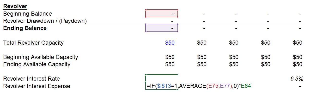
Once we link the interest expense back into the FCF forecast, a Circularity will be introduced into our model. Therefore, we have added a circularity toggle in case the model breaks.

Basically, what the formula above is saying is:

• If the toggle is switched to “1”, then the average of the beginning and ending balance will be taken
• If the toggle is switched to “0”, then a zero will be output, which removes all the cells populated with “#VALUE” (and can be toggled back to use the average)

Finally, the revolver comes with an unused commitment fee, which is 0.25% in this scenario. To calculate this annual commitment fee, we multiply this 0.25% fee by the average of the beginning and ending available revolver capacity, since this represents the revolver amount not being used.

Term Loan B (“TLB”)

Moving onto the next tranche in the waterfall, the Term Loan B will be forecasted in a similar roll-forward but this schedule will be simpler given our model assumptions.

The only factor that impacts the ending TLB balance is the scheduled principal amortization of 5%. For each year, this will be calculated as the total amount raised (i.e. the principal) multiplied by the 5% mandatory amortization.

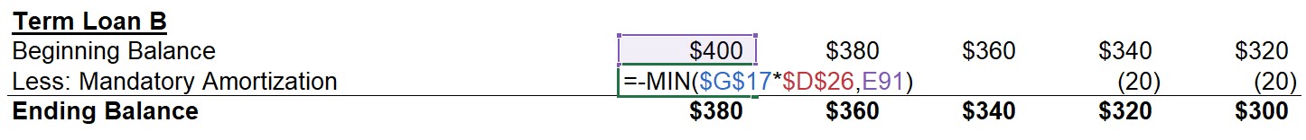
While it is less relevant to this scenario, we have wrapped a “-MIN” function to output the lesser number between the (Principal * Mandatory Amortization %) and the Beginning TLB Balance. This prevents the principal amount paid down from exceeding the balance remaining.

For example, if the required amortization was 20% per year and the holding period was 6 years, without this function in place – JoeCo would still be paying the mandatory amortization in year 6 despite the principal being fully paid off (i.e. the beginning balance in Year 6 would be zero, so the function will output the zero rather than the mandatory amortization amount)

The amortization amount is based on the original debt principal regardless of how much of the debt has been paid down to date.

In other words, the mandatory amortization of this TLB will be $20mm each year until the remaining principal will be due in one final payment at the end of its maturity.

The interest rate calculation for TLB is shown below:

The formula is the same as the revolver, but this time there is a LIBOR floor of 2%. Since LIBOR is 1.5% in 2021, the “MAX” function will output the larger number between the floor and LIBOR – which is the 2% floor for 2021.

The 2nd part is the spread of 400 basis points divided by 10,000 to arrive at 0.04, or 4.0%.

Given how LIBOR is 1.5% in 2021, the TLB interest rate will be calculated as 2.0% + 4.0% = 6.0%.

Then, to calculate the interest expense – we take the TLB interest rate and multiply it by the average of the beginning and ending TLB balance.

Notice how as the principal is paid down, the interest expense decreases. Contrast this to mandatory amortization, in which the amount paid remains constant regardless of the principal paydown.

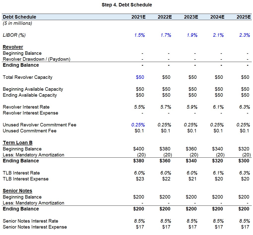
The approximate interest expense is ~$23mm in 2021 and falls to ~$20mm by 2025.

However, this dynamic is less apparent in our model given the mandatory amortization is only 5.0% and we are assuming no cash sweeps (i.e. prepayment using excess FCF is not allowed).

Senior Notes

Relative to equity and other riskier notes/bonds that the PE firm could have potentially used as funding sources, Senior Notes are higher up in the capital structure and considered to be a “safe” investment from the perspective of most lenders. However, Senior Notes are still below bank debt (e.g. Revolver, TLs) and usually unsecured despite the name.

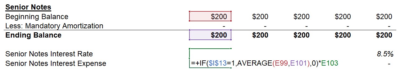
One characteristic of these Senior Notes is that there will be no required principal amortization, meaning the principal will not be paid until maturity.

We saw how with the TLB, the interest expense (i.e. the proceeds to the lender) decreases as the principal is gradually paid down. So, the lender of the Senior Notes chose to neither require any mandatory amortization nor allow prepayment.

As you can see below, the interest expense is $17mm each year, and the lender receives an 8.5% yield on the $200mm outstanding balance for the entire tenor.

Forecast Completion

The debt schedule is now done, so we can return to the parts of the FCF forecast that we skipped over and left blank.

• Interest Expense: The interest expense line item will be calculated as the sum of all of the interest payments from each debt tranche, as well as the unused commitment fee on the revolver.
• Mandatory Amortization: In order to complete the forecast, we will link the mandatory amortization amount due from the TLB directly to the “Less: Mandatory Amortization” line item on the forecast, right above the “Free Cash Flow (Pre-Revolver)”.

For more complex (and realistic) transactions where various debt tranches require amortization, you would take the sum of all of the amortization payments due that year and then link it back to the forecast.

Our free cash flow projection model is now complete with those two final linkages made.

Step 4: Formulas Used

• Available Revolver Capacity = Total Revolver Capacity – Beginning Balance
• Revolver Drawdown / (Paydown): “=MIN (Available Revolver Capacity, –MIN (Beginning Revolver Balance, Free Cash Flow Pre-Revolver)”
• Revolver Interest Rate: “= MAX (LIBOR, Floor) + Spread”
• Revolver Interest Expense: “IF (Circularity Toggle = 1, AVERAGE (Beginning, Ending Revolver Balance), 0) × Revolver Interest Rate
• Revolver Unused Commitment Fee: “IF (Circularity Toggle = 1, AVERAGE (Beginning, Ending Available Revolver Capacity), 0) × Unused Commitment Fee %
• Term Loan B Mandatory Amortization = TLB Raised × TLB Mandatory Amortization %
• Term Loan B Interest Rate: “= MAX (LIBOR, Floor) + Spread”
• Term Loan B Interest Expense: “IF (Circularity Toggle = 1, AVERAGE (Beginning, Ending TLB Balance), 0) × TLB Interest Rate
• Senior Notes Interest Expense = “IF (Circularity Toggle = 1, AVERAGE (Beginning, Ending Senior Notes), 0) × Senior Notes Interest Rate
• Interest = Revolver Interest Expense + Revolver Unused Commitment Fee + TLB Interest Expense + Senior Notes Interest Expense

As a side note, one common feature in LBO models is a “cash sweep” (i.e. optional repayments using excess FCFs), but this was excluded in our basic model. For this reason, the “Free Cash Flow (Post-Revolver)” will be equal to the “Net Change in Cash Flow” since there are no more uses of cash.

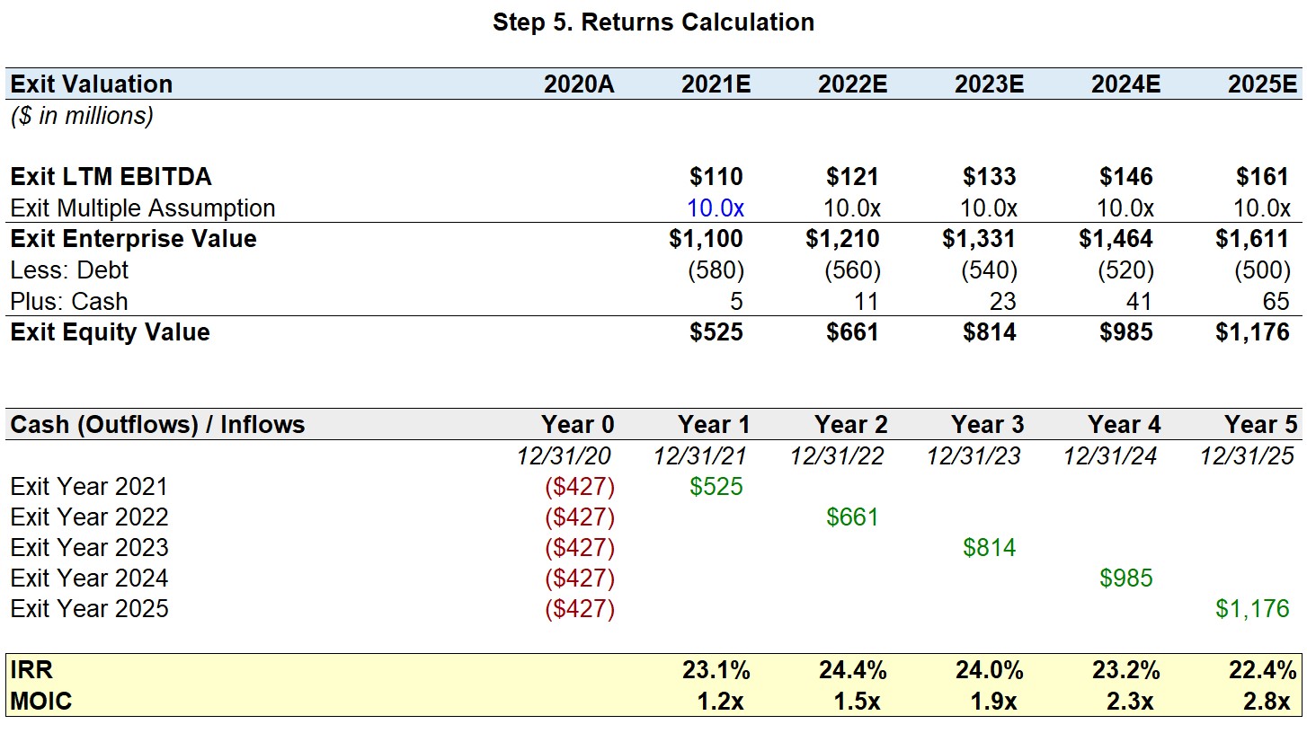
Step 5. Returns Calculation

Exit Valuation

Now that we have projected the financials of JoeCo and the net debt balance for the five-year holding period, we have the necessary inputs to calculate the implied exit value for each year.

• Exit Multiple Assumption: The first input will be the “Exit Multiple Assumption”, which was stated as being the same as the entry multiple, 10.0x.
• Exit EBITDA: In the next step, we’ll create a new line item for “Exit EBITDA” which simply links to the EBITDA of the given year. We will grab this figure from the FCF forecast.
• Exit Enterprise Value: We can now calculate the “Exit Enterprise Value” by multiplying the Exit EBITDA by the Exit Multiple Assumption.
• Exit Equity Value: Similar to how we did in the first step for the entry valuation, we will then deduct the net debt from the enterprise value to arrive at the “Exit Equity Value”. The total debt amount is the sum of all of the ending balances in the debt schedule, while the cash balance will be pulled from the cash roll forward in the FCF forecast (and Net Debt = Total Debt – Cash)

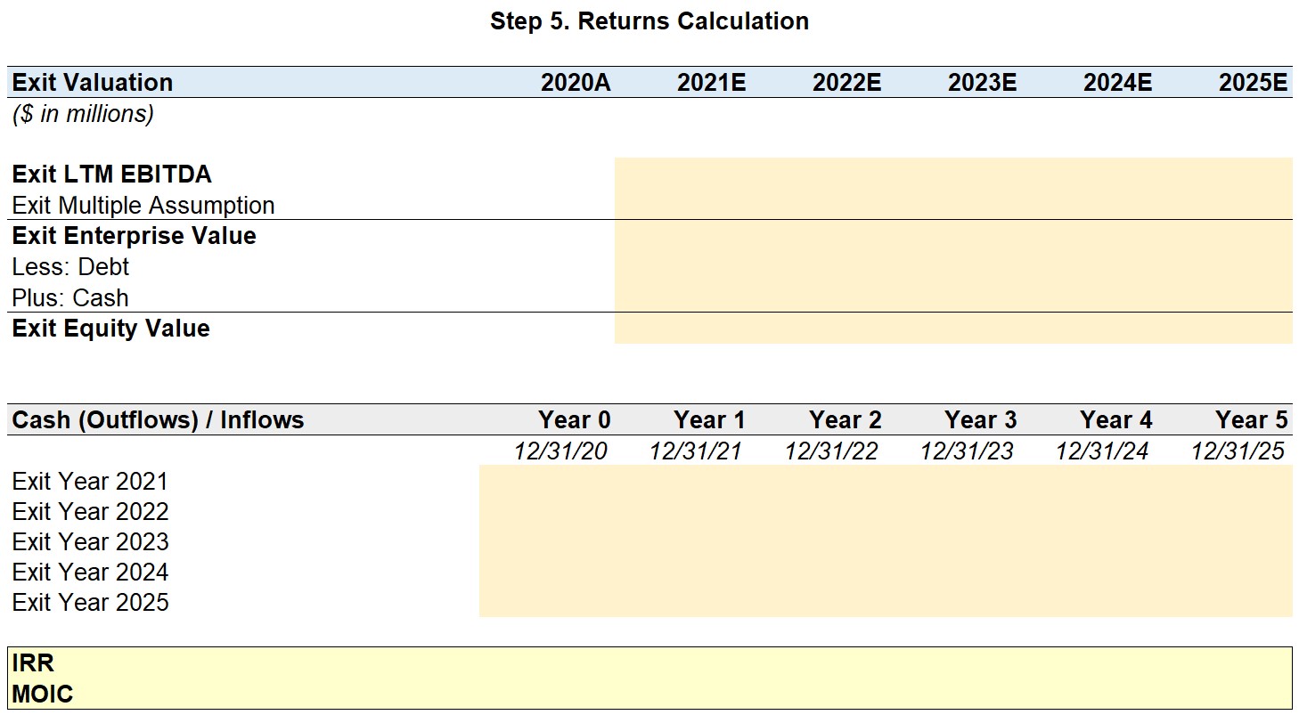
Internal Rate of Return (IRR)

In the final step, we will calculate the two return metrics we were instructed to by the prompt:

1. Internal Rate of Return (IRR)
2. Cash-on-Cash Return (aka MOIC)
   

Starting with the internal rate of return (IRR), to determine the IRR of this investment in JoeCo, you first need to gather the magnitude of the cash (outflows) / inflows and the coinciding dates of each.

The initial equity contribution by the financial sponsor needs to be inputted as a negative since the investment is an outflow of cash. In contrast, all-cash inflows are inputted as positives. But in this case, the only inflow will be the proceeds received from the exit of JoeCo.

Once the “Cash (Outflows) / Inflows” section has been completed, enter “=XIRR” and drag the selection box across the entire range of cash (outflows) / inflows in the relevant year, insert a comma, and then do the same across the row of dates. The dates must be formatted correctly for this to work properly (e.g. “12/31/2025”, rather than “2025”).

Multiple on Invested Capital (“MOIC”)

The multiple-on-invested-capital (MOIC), or “cash-on-cash return”, is calculated as the total inflows divided by the total outflows from the perspective of the PE firm.

Since our model is less complex with no other proceeds (e.g. dividend recaps, consulting fees), the MOIC is the exit proceed divided by the $427 initial equity investment.

To perform this in Excel, use the “SUM” function to add up all the inflows received during the holding period (green font), and then divide by the initial cash outflow in Year 0 (red font) with a negative sign in front.

Step 5: Formulas Used

• Exit Enterprise Value = Exit Multiple × LTM EBITDA
• Debt = Revolver Ending Balance + Term Loan B Ending Balance + Senior Notes Ending Balance
• IRR: “= XIRR (Range of Cash Flows, Range of Timing)”
• MOIC: “=SUM (Range of Inflows) / – Initial Outflow”

Conclusion of LBO Model Test Guide

If we assume an exit in Year 5, the private equity firm was able to 2.8x from its initial equity investment in JoeCo and achieve an IRR of 22.5% throughout the holding period.

• Internal Rate of Return (IRR) = 22.4%
• Multiple on Invested Capital (MOIC) = 2.8x

In closing, our basic LBO modeling test tutorial is now complete, so we hope the instructions were intuitive, and stay tuned for the next post in our LBO modeling series.