
- What is CAPM?
- How Does Capital Asset Pricing Model Work?
- What are the CAPM Theory Assumptions?
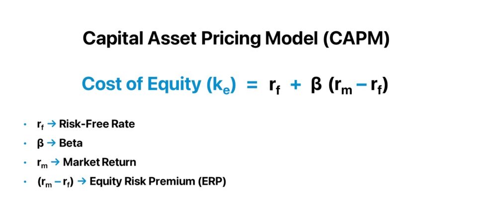
- CAPM Formula
- CAPM Calculation Example
- What is the Full-Form CAPM Equation?
- CAPM Theory Graph: Expected Return vs. Risk Trade-Off
- CAPM Calculator — Excel Template
- 1. Illustrative CAPM Calculation Example
- 2. Expected Return Calculation Example
What is CAPM?
The Capital Asset Pricing Model (CAPM) estimates the expected return on an investment based on the perceived systematic risk. The cost of equity—the required rate of return for equity holders—is calculated using the CAPM.
- CAPM stands for “Capital Asset Pricing Model” and measures the cost of equity (Ke), or expected rate of return, on a particular security or portfolio.
- The CAPM formula is equal to the risk-free rate (rf) plus the product between beta (β) and the equity risk premium (ERP).
- The CAPM establishes the relationship between the risk-return profile of a security (or portfolio of securities) based on the risk-free rate (rf), beta (β), and equity risk premium (ERP).
- CAPM calculates the cost of equity, or expected return on equity, which is a core component of the weighted average cost of capital (WACC).
How Does Capital Asset Pricing Model Work?
The capital asset pricing model (CAPM) is a fundamental method in corporate finance to determine the required rate of return on an equity investment given the coinciding risk profile.
In short, the CAPM establishes the relationship between the risk and expected return on an equity security based on three underlying variables:
- Risk-Free Rate (rf)
- Beta (β) of the Underlying Security
- Equity Risk Premium (ERP)
However, the discount rate concept must be comprehended to understand the core components of the capital asset pricing model (CAPM) theory.
The discount rate represents the “hurdle rate” on an investment or project—i.e. the minimum rate of return corresponding to the risk profile, which could refer to share issuances by a publicly-traded company or a proposed project that a corporation is under consideration on whether to proceed.
To perform a cash flow-oriented valuation on a company, the implied intrinsic value equals the sum of its future cash flows discounted to their present value (PV) using an appropriate discount rate.
Under the specific context of equity investors, the discount rate that pertains solely to common shareholders is referred to as the “cost of equity,” which is the required rate of return to equity investors that the capital asset pricing model is used to calculate.
The unlevered free cash flow, or free cash flow to firm (FCFF), is generated by a company and discounted using the weighted average cost of capital (WACC), whereas levered free cash flow or free cash flow to equity (FCFE) is discounted using the cost of equity (ke).
- Free Cash Flow to Firm (FCFF) → Weighted Average Cost of Capital (WACC)
- Free Cash Flow to Equity (FCFE) → Cost of Equity (Ke)
But regardless of the type of cash flow being discounted, the cost of equity (ke) serves an integral role in either approach because it is an input in the WACC formula.
What are the CAPM Theory Assumptions?
Under Modern Portfolio Theory (MPT), there are two core assumptions that underpin the capital asset pricing model (CAPM):
- Efficient Markets (Competitive) ➝ The financial markets are competitive and efficient in terms of information collection, which impacts the pricing of securities in the markets – identifying mispricings in the market is becoming increasingly challenging.
- Rational Investors (Risk-Averse) ➝ The participants in the financial markets are assumed to be rational, risk-averse investors for the most part.
The cost of equity (ke) is most commonly estimated using the capital asset pricing model (CAPM), which connects the expected return on security (or portfolio of securities) to its sensitivity to the broader market.
CAPM Formula
The capital asset pricing model (CAPM) formula states that the cost of equity—the return expected to be earned by common shareholders—is equal to the risk-free rate (rf) plus the product of beta and the equity risk premium (ERP).
Where:
- Ke ➝ Cost of Equity (or Expected Return)
- rf ➝ Risk-Free Rate
- β ➝ Beta
- (rm – rf) ➝ Equity Risk Premium (ERP)
CAPM Calculation Example
Suppose we’re computing the cost of equity (ke) using the CAPM given the following set of assumptions:
CAPM Exercise Assumptions
- Risk-Free Rate (rf) = 3.0%
- Beta (β) = 0.8
- Expected Market Return (rm) = 10.0%
- Equity Risk Premium (ERP) = 10.0% – 3.0% = 7.0%
By entering the provided assumptions into the CAPM formula, we arrive at a cost of equity (ke) of 8.6%.
- Cost of Equity (Ke) = 3% + 0.8 (7.0%) = 8.6%
What is the Full-Form CAPM Equation?
The capital asset pricing model (CAPM) equation is composed of three components:
- Risk-Free Rate (rf) → The return received from risk-free investments — most often proxied by the 10-year treasury yield
- Beta (β) →The measurement of the volatility (i.e. systematic risk) of a security compared to the broader market (S&P 500)
- Equity Risk Premium (ERP) → The incremental return received from investing in the market (S&P 500) above the risk-free rate (rf, as described above)
Component 1. Risk-Free Rate (rf)
Starting off, the risk-free rate (rf) should theoretically reflect the yield to maturity (YTM) of default-free government bonds of equivalent maturity to the duration of each cash flow being discounted.
However, due to the lack of liquidity in government bonds with the longest maturities (i.e. less trade volume and data sets), the current yield on 10-year US treasury notes has become the standard proxy for the risk-free rate assumption for companies based in the US.
Component 2. Beta (β)
In corporate finance, beta (β) measures the systematic risk of a security compared to the broader market (i.e. non-diversifiable risk).
The beta of an asset is calculated as the covariance between expected returns on the asset and the market, divided by the variance of expected returns on the market.
The relationship between beta (β) and the expected market sensitivity is as follows:
- β = 0: No Market Sensitivity
- β < 1: Low Market Sensitivity
- β = 1: Same as Market (Neutral)
- β > 1: High Market Sensitivity
- β < 0: Negative Market Sensitivity
For instance, a company with a beta of 1.0 would expect to see returns consistent with the overall stock market returns. So if the market has gone up by 10%, the company should also see a return of 10%.
But if that company were to have a beta of 2.0, it would expect a return of 20%, assuming the market had gone up by 10%.
- Systematic Risk ➝ Often referred to as market risk, systematic risk is inherent to the entire equities market, as opposed to being specific to a particular company or industry. In short, systematic risk is unavoidable and cannot be mitigated through portfolio diversification (e.g. global recessions).
- Unsystematic Risk ➝ Unsystematic risk refers to the company-specific (or industry-specific) risk that can actually be reduced through portfolio diversification (e.g. supply chain shutdowns, lawsuits). The benefits of diversification become more profound if the portfolio contains investments in different asset classes, industries, and geographies.
The common source of criticism is most often related to beta, as many criticize the metric as a flawed measure of risk.
- Trailing-Basis ➝ The standard procedure for estimating the beta of a company is through a regression model that compares the historical market index returns and company-specific returns, in which the slope of the regression line corresponds to the beta of the company’s shares (the calculation is thus “backward-looking”). However, the past performance (and correlation) of a company relative to the market may not be an accurate indicator of future share price performance.
- Capital Structure Mix ➝ The capital structure (debt/equity ratio) of companies also progressively changes over time, which can alter their risk profiles and performance.
Component 3. Equity Risk Premium (ERP)
Our third input, the equity risk premium (ERP), or “market risk premium,” measures the incremental risk (or excess return) of investing in equities over risk-free securities.
Since investing in risky assets such as equities comes with additional risk (i.e. potential for loss of capital), the equity risk premium serves as additional compensation for investors to have an incentive to take on the risk.
The equity risk premium has been around the 4% to 6% range, based on historical spreads between the S&P 500 returns over the yields on risk-free government bonds.
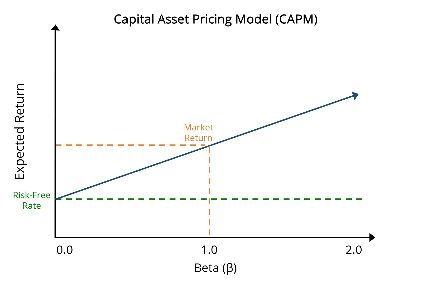
CAPM Theory Graph: Expected Return vs. Risk Trade-Off
The following graph of the capital asset pricing model (CAPM) illustrates the relationship between expected returns (y-axis) and beta (x-axis).
- Green Dotted Line → Risk-Free Rate (rf)
- Orange Dotted Line → Market Return
- Navy Line → Security Market Line (SML)
- X-Axis → Beta (β)
- Y-Axis → Expected Return, E(R), or Cost of Equity (ke)
The difference between the yield earned on the risk-free rate and the market return represents the equity risk premium (ERP).
If plotted on a chart, the capital asset pricing model (CAPM) depicts the relationship between the expected return and trade-off with regard to risk.
The CAPM graph implies the expected returns (i.e. the y-axis) rise in tandem as more risk is undertaken by the investor (i.e. the x-axis), and vice versa.
Note: The market beta is equal to 1.0 here.
Capital Asset Pricing Model Graph (CAPM)
CAPM Calculator — Excel Template
We’ll now move on to a modeling exercise, which you can access by filling out the form below.
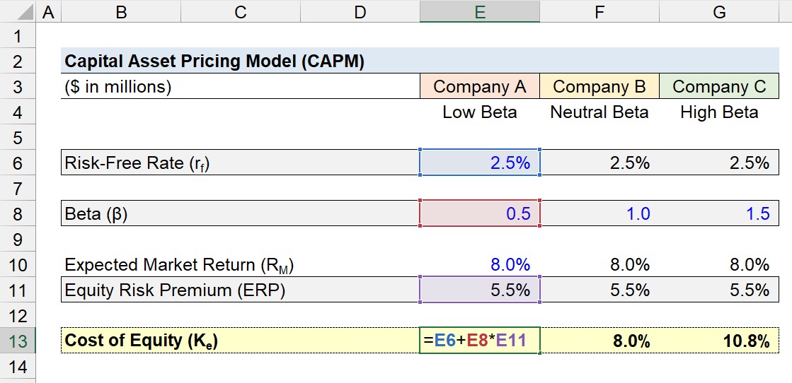
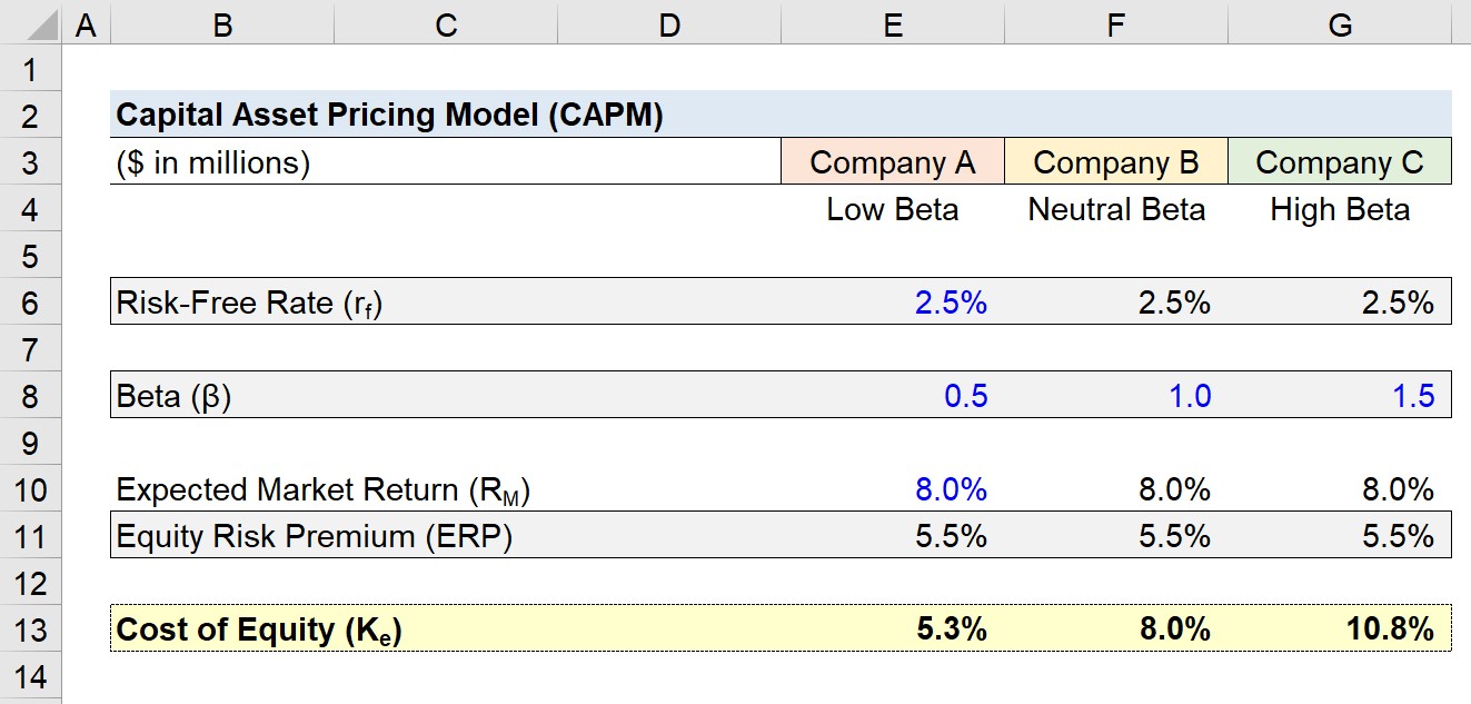
1. Illustrative CAPM Calculation Example
Suppose we have three companies that each share the following assumptions:
- Risk-Free Rate (rf) = 2.5%
- Expected Market Return = 8.0%
Since we’re given the expected return on the market and risk-free rate, we can calculate the equity risk premium (ERP) for each of the three companies using the formula below:
- Equity-Risk Premium (ERP) = 8.0% – 2.5% = 5.5%
The difference in expected returns among the three companies will be attributable to the beta (i.e. systematic risk).
- Beta (β), Company A = 0.5
- Beta (β), Company B = 1.0
- Beta (β), Company C = 1.5
To calculate the cost of equity (Ke), we’ll take the risk-free rate and add it to the product of beta and the equity risk premium, with the ERP calculated as the expected market return minus the risk-free rate.
For example, Company A’s cost of equity can be calculated using the following equation:
- Cost of Equity (Ke) = 2.5% + (0.5 × 5.5%) = 5.3%
Under the provided assumptions, the expected equity returns for the three companies come out to 5.3%, 8.0%, and 10.8%, respectively.
- Cost of Equity (Ke), Company A = 5.3%
- Cost of Equity (Ke), Company B = 8.0%
- Cost of Equity (Ke), Company C = 10.8%
2. Expected Return Calculation Example
In the final section of our practice exercise in Excel, we’ll review the core concepts covered in our illustrative cost of equity calculation using the capital asset pricing model (CAPM):
- Lower Beta = Lower Potential Returns (and Risk) ➝ The lowest the potential returns (and risk) attributable to a particular investment, the lower the beta
- Market Beta = 1.0 ➝ The returns earned on a security with a beta of 1.0 will exhibit return in line with that of the broader market (S&P)
- Higher Beta = Greater Potential Returns (and Risk) ➝ The company with the highest potential returns (and risk) has the highest beta
In conclusion, a company with a high beta implies increased risk and higher volatility relative to the overall market (i.e. greater sensitivity to market fluctuations).
Therefore, a higher cost of equity would be used by investors to discount the future cash flows generated by the company, causing a reduction to the implied valuation, all else being equal.
Everything You Need To Master Financial Modeling
Enroll in The Premium Package: Learn Financial Statement Modeling, DCF, M&A, LBO and Comps. The same training program used at top investment banks.
Enroll Today")


Using the CAPM Model, how do you rearrange to work out the Rf rate?
can the beta of a security, Bi be substituted for the beta of a portfolio? or would the beta of a portfolio be the sum of weighted beta’s (portfolio weighting x individual beta)
The beta used here is the ‘levered’ beta, right?
To calculate the CAPM,risk-free rate and add it to the product of beta and the equity risk premium, with the CAPM calculated as the expected market return minus the risk-free rate.
HI, If we have to make a valuation for another 5 years on a company based on the above formula, where to look for the data and values I mean which sheets should I look for
why is risk-free rate considered in calculating capm?