
- Advanced LBO Modeling Test: Training Guide
- Advanced LBO Modeling Test: Practice 4-Hour Tutorial
- LBO Modeling Test Format: Advanced Edition
- Advanced LBO Modeling Test — Excel Template
- Advanced LBO Modeling Test Illustrative Prompt
- Step 1. Model Assumptions
- Step 2. Sources and Uses Table
- Step 3. Purchase Price Allocation (PPA)
- Step 4. Closing B/S Adjustments
- Step 5. Add-On Financial Build
- Step 6. Pro Forma Financial Forecast
- Step 7. Management Contingency Payments
- Step 8. Debt Schedule
- Step 9. Capitalization Table
- Step 10. Returns Calculation
- LBO Modeling Tutorial Conclusion
Advanced LBO Modeling Test: Training Guide
The following Advanced LBO Modeling Test training guide provides a step-by-step tutorial to complete a 3-hour practice LBO modeling test of advanced difficulty in Excel.

Advanced LBO Modeling Test: Practice 4-Hour Tutorial
If you are capable of completing all four levels of difficulties covered in our modeling series (Paper LBO, Basic LBO, Standard LBO, and Advanced LBO) without reliance on the templates, you should rest assured knowing that you have the necessary foundation to complete the vast majority of LBO tests handed out in private equity interviews.
The following modeling test is the final post in our five-part series on private equity interviews and LBO modeling tests:
- Top 25 Private Equity Interview Questions — Confirms that you have the baseline knowledge of the technical aspects expected of a potential candidate
- Paper LBO Test — Given at earlier rounds, you’ll get a pen and paper (no calculator) and 5-10 minutes
- Basic LBO Modeling Test — You’re given a laptop, simple instructions and ~30 minutes – this serves as a slightly more robust early-round screen than the Paper LBO
- Standard LBO Modeling Test — You’re given a laptop and around 1-2 hours – this is the most common LBO modeling test given at lower-middle market and middle-market PE firms.
- Advanced LBO Modeling Test (*This Post*) – You’re given a laptop, a 5-15 page packet of financial data, and 3 to 4 hours. You’re more likely to see this from upper-middle market firms or mega-funds in the later rounds of the interview process. The exception is if the process is rushed for that particular recruiting cycle.
Just to list out a few of the more challenging topics covered here, integrated into this specific leveraged buyout model is a dividend recapitalization, convertible preferred equity investment structure, original issuance discounts (OIDs), add-on acquisitions, contingency management compensation, and more.
Once you feel adequately prepared for all levels of modeling tests, your remaining preparation time should be allocated towards practicing under similar time-pressured conditions and gaining sector-specific knowledge based on the firm you’re interviewing with other tasks, such as:
- General News (e.g. WSJ, Financial Times)
- Industry-Specific Articles
- Industry Primers (e.g. Pitchbook, Bain PE Report)
- Initiating Coverage Equity Research Reports
LBO Modeling Test Format: Advanced Edition
Throughout our guide, we explain concepts likely to be tested during LBO modeling tests on the more difficult end of the spectrum.
We tried our best to balance quantity and depth, and covered every concept to the point that you should be able to understand it well enough to figure it out on your own during the interview.
Below is a summary of what you’ll see and how it compares to the Standard LBO Modeling Test:
| Standard LBO Modeling Test | Advanced LBO Modeling Test | |
| Test Format |
|
|
| Time Allotted |
|
|
| Scoring Criteria |
|
|
| Concepts Tested | The standard LBO Model Test will usually include the following elements – this is the “bread & butter” of an LBO modeling test:
|
The advanced LBO modeling test is essentially the standard LBO modeling test + any of the following features:
Note: It is very unlikely for a candidate to be asked to model all these features in a single LBO model test. |
The model we will build together should take you less than 3 hours, not 4 hours. That’s because we will provide you with all the relevant assumptions in a convenient format (Excel) rather than the PDF or Word document you’d get in the test, forcing you to manually input the historical data, which usually amounts to 30-40 extra minutes of work.
The assumptions used for the different cases are rarely provided in the format we will. In most modeling tests, you will be given the CIM, which contains the management projections. It is up to your discretion whether to use this as your “Base Case” or to adjust it as you feel necessary.
Sometimes, you might even find a supplementary industry report (just a few pages) inside the packet to help you determine your assumptions for all the cases. Otherwise, the firm will expect you to understand the unit economics of the industry, and adjust your assumptions accordingly, without any external resources.
You might also be surprised to hear that, unlike our Standard LBO Modeling test, where you have to build a full 3-statement model, you will not be asked to do so here. The concepts tested in advanced LBOs tend to cause modeling the balance sheet to be unnecessarily complicated given the time allotment.
For example, you might be asked to model an add-on’s impact on the internal rate of return (IRR), but not to create another closing B/S for that add-on transaction and then integrate it into the platform’s B/S forecast.
The Wharton Online and Wall Street Prep Private Equity Certificate Program
Level up your career with the world's most recognized private equity investing program. Enrollment is open for the Feb. 10 - Apr. 6 cohort.
Enroll TodayAdvanced LBO Modeling Test — Excel Template
We’ll now move to our advanced LBO modeling test, which you can access by filling out the form below.
Advanced LBO Modeling Test Illustrative Prompt
Situational Overview
A private equity firm (“Lead Sponsor”) is in the process of the take-private leveraged buyout of JoeCo, a publicly-traded coffee company. The latest closing price of JoeCo was $14.25 per share, but JoeCo’s shareholder board and shareholders had pre-determined $12.00 as the basis of the takeout offer. The takeout offer value per share was a 25% premium over the normalized share price.
The private equity firm leading the deal has offered Wall Street Prep Capital Partners (“WSPCP”) the opportunity to co-invest into the deal via a preferred equity investment into JoeCo. The amount invested would be $475mm and the preferred equity will PIK at an 8.5% accrual rate with the optionality to convert. Also, WSPCP would be receiving a $5mm monitoring fee each year for its consulting services to JoeCo.
The remaining equity contribution required will be funded entirely by the Lead Sponsor in the form of common equity. To pitch the deal, the Lead Sponsor has mentioned two potential levers to increase equity returns, 1) the add-on acquisition of TeaCo and 2) a dividend recapitalization.
The Lead Sponsor has mentioned that its ideal plan is to acquire TeaCo in 2021 and then to complete a dividend recap in 2024. The reason is, the Lead Sponsor expects JoeCo to perform inline with its base case, whereas TeaCo has a high likelihood of outperforming and following the upside case.
In terms of the exit, the Lead Sponsor has indicated that it is under the belief that the two firms would be able to exit to a strategic at a multiple near the entry multiple.
Based on the lender agreements, the sponsors are restricted from issuing themselves a dividend for the first two years and the maximum leverage that the additional debt can be raised up to is a total leverage multiple of 6.0x (i.e. based on the initial leverage multiple). In addition, the interest coverage ratio (EBITDA / Interest Expense) must remain above 2.0x throughout all years.
Instructions: Using the information provided and the assumptions listed below, create a functional forecast model that calculates the returns to WSPCP from this potential co-investment in JoeCo.
Transaction Assumptions
- The normalized share price of JoeCo is $12.00 and a 25% premium will be the takeout offer
- JoeCo has 315mm basic shares outstanding and three tranches of options (1mm @ $3.00, 2mm @ $5.00, and 2.5mm @ $10.00)
- The transaction fee paid will be 2.5% of the total offer equity value
- The Cash to B/S must be $25mm and all existing debt will be refinanced upon deal closure
- JoeCo’s Intangible Assets will be written up 10% with a useful life assumption of 15 years
- JoeCo’s PP&E will be written up 10% with a useful life assumption of 8 years
- Upon closing of the deal on 12/31/2020, the share price of JoeCo will be adjusted to a dollar basis (i.e. each common share will be worth $1.00)
- Use a tax rate of 25%
Financing Assumptions
- The revolver was left undrawn at purchase, priced at LIBOR + 400, maximum revolver capacity of $1,000mm, and an unused revolver commitment fee of 0.25%
- Unitranche Term Loan was raised at 6.0x of LTM EBITDA, issued 99 of par, and priced at LIBOR + 400 with a 1% floor, 5% mandatory amortization, and full cash sweep
- Assume the financing fees amortization period is 8 years for all periods and a financing fee of 2% for all debt tranches (excluding the revolver)
Investment Assumptions
- WSPCP’s investment is of preferred convertible equity and the total investment amounts to $475mm with a PIK accrual rate of 8.5%
- The conversion strike price on the WSPCP’s investment is $1.25
- A 5% management option pool was reserved with the strike price being issued in-the-money (“ITM”) at $1.00
Management Contingency Payments Assumptions
- There will be contingency-based management compensation if certain EBITDA targets are met, there will be three levels and the maximum that can be earned is $10mm each year (minimum @ $2mm, midpoint @ $3mm, and outperformance @ $5mm)
- The minimum EBITDA target in 2021 was set at $350mm and each year the target will increase by 15% YoY
- The midpoint and outperformance will be 10% higher than one another, and will similarly increase by 15% YoY
Add-On Assumptions
- The Lead Sponsor believes it can acquire TeaCo at 9.5x LTM EBITDA
- Funding for the acquisition will come from JoeCo’s FCF and the revolver
- For the add-on acquisition, the institutional lender has agreed to provide a revolving line of credit of $1,000mm
- There is no restriction on the year that TeaCo could be acquired
- In 2020, TeaCo generated $100mm in Revenue, $30mm in Gross Profit, $10mm in SG&A, and $5mm in R&D – for an EBITDA of $15mm
- TeaCo in 2020 had 250 stores in the U.S. with 50,000 annual orders per store
- TeaCo has no D&A or other sources of income / (expenses)
- Assume there are no revenue or cost synergies from the add-on, and ignore tax implications
Dividend Recap Assumptions
- Additional debt raised for the dividend recap will in the form of bonds with a fixed interest rate of 8.5%, no required amortization, and NC/L (i.e. no prepayment allowed for life)
- If a dividend recap is to be completed, it will be completed right at the beginning of the year
- In terms of how the dividend will be distributed between the Lead Sponsor and WSPCP, the percentages will be based on the initial equity contributions at purchase
Note: The LTM financials of JoeCo and TeaCo, and the assumptions for the key drivers of each company are included in the first sheet of the model template.
Step 1. Model Assumptions
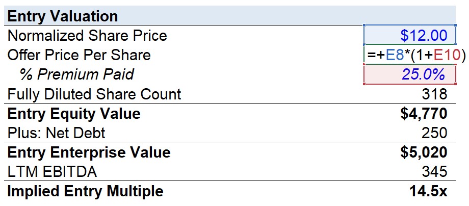
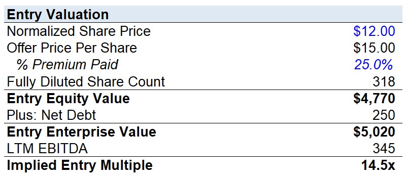
Entry Valuation
In our LBO model, the entry valuation is based on the $15.00 offer price per share, rather than an EV/EBITDA multiple, given that JoeCo is a publicly-traded company. We can arrive at the pre-deal share price of $12.00 as $15.00/(1+25%).
In the next step, we’ll move to equity value, which will require us to determine the total share count.
To calculate the fully diluted shares outstanding, the Treasury Stock Method (TSM) is used, which includes all dilutive securities (restricted stock and in-the-money options) in the share count, but assumes the option proceeds are used by the company to buy back shares to mitigate the dilutive impact.
The calculation of net dilution for each option tranche is as follows.
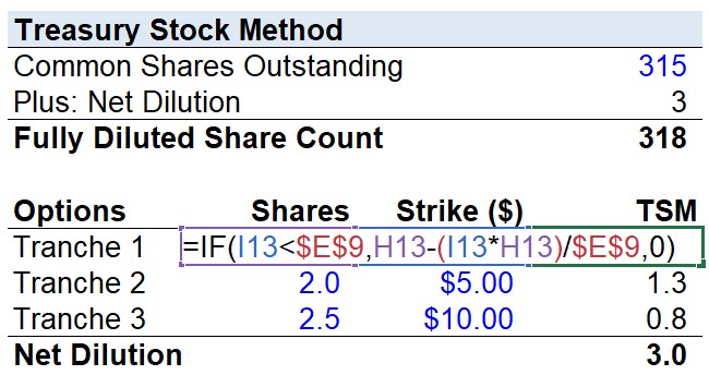
So while the prompt tells us there are 5.5 million options, the treasury stock method calculates the option proceeds for each tranche of options and calculates how many shares can be bought back at the offer price. Therefore, we see the net dilutive impact is only 3.0 million shares, not 5.5 million.
To calculate the dilutive impact under the TSM, we’ll first insert an “IF” function that says if the strike price is below the offer price per share, then all the options in the tranche will be exercised by the holders, which are often employees and management (i.e. stock-based compensation). But the option holders’ end of the bargain is to pay JoeCo for each share price at the strike price as part of the contract.
Under the TSM, we assume JoeCo will use those proceeds received to repurchase shares to minimize dilution. The number of shares repurchased will be calculated by multiplying the number of new shares by the strike price and then dividing that by the offer share price of $15.00.
After doing the TSM calculation for each tranche, we can sum up the three tranches and see the net dilution impact was 3.0mm shares. The fully diluted shares outstanding of JoeCo are thus 318mm.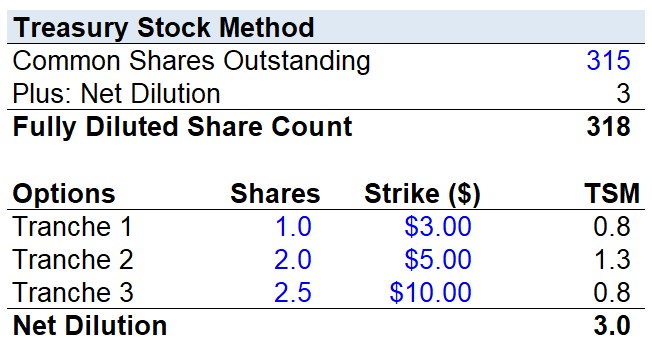
Now that we have the diluted share count, the entry equity value can then be calculated by multiplying the offer price per share of $15.00 by the fully diluted share count we just calculated, which gets us to $4,770mm.
- Net Debt: JoeCo’s pre-deal balance sheet has $450mm in gross debt and $200mm in cash, for net debt of $250mm.
- Implied Entry Multiple (EV/EBITDA): To back into our implied purchase entry multiple, we will add the net debt of $250mm to arrive at an entry enterprise value of $5,020mm, and then divide that by JoeCo’s LTM multiple of $345mm to arrive at 14.5x as the implied entry multiple (EV/EBITDA) paid to take JoeCo private.
Entry Offer Price vs. Entry Multiple
In the prompt, we were given an offer price as the initial valuation input, which led us to equity value directly, from which we’ll add net debt to determine JoeCo’s entry enterprise value.
If JoeCo were a private company, the explicit entry valuation assumption would be the EV/EBITDA multiple, which would arrive at enterprise value directly, from which we would subtract net debt to get to equity value.
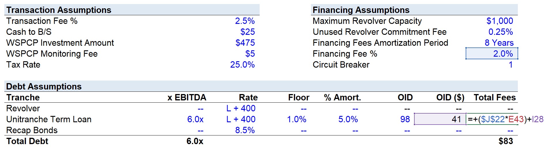
Transaction Assumptions
With the initial valuation done, we will now lay out some of the key transaction and financing assumptions provided in the Prompt – beginning with the “Transaction Assumptions“:
![]()
- Transaction Fees: The transaction fee assumption was 2.5% of the offer equity value, which we’ll soon multiply by the entry equity value of $4,770mm to calculate $119mm in transaction fees
- Cash to Balance Sheet: We assume JoeCo will require $25mm on the B/S at the closing of the transaction
- Monitoring Fees: An annual monitoring fee of $5mm will be paid exclusively to WSPCP – this sponsor consulting fee will not be divided among all the equity owners as it is compensation for the services provided by the consulting arm of WSPCP
- Tax Rate: The final assumption for this section is the 25% tax to be used throughout the entirety of the model
Financing Assumptions
First off on our financing assumptions, the maximum revolver capacity is stated as $1,000mm. We can infer that WSPCP and the 2nd Sponsor were able to negotiate and obtain a revolver of this magnitude due to JoeCo’s past profitability and credit rating.
The next three financing assumptions are straightforward and simple hard codes:
- Unused Commitment Fee: The unused revolver commitment fee is 0.25%
- Financing Fees Amortization: The number of periods in which the financing fees are amortized is 8 years
- Financing Fees: The financing fee is 2.0% for all the debt tranches, excluding the revolver
Unlike a traditional asset-backed revolver, which is tied to a borrowing formula based on a percentage of the borrowers’ inventory and A/R balance, this revolver is unsecured by collateral and based on the future cash flows of JoeCo (i.e. cash-flow based revolver).
The institutional lender that provided the revolver and unitranche term loan was made aware of the sponsors’ plan to make an add-on acquisition and perform a dividend recap and therefore provided this line of credit to ensure JoeCo has sufficient liquidity available (i.e. “cushion”).
Debt Assumptions
We will now turn to the debt assumptions.
- Revolver: Left undrawn at purchase and is priced at a floating rate of “LIBOR + 400” with no floor.
- Unitranche Term Loan: Rather than having senior and junior tranches of debt in the capital structure, an increasingly popular financing structure is unitranche debt, in which the total unitranche debt raised was 6.0x LTM EBITDA.
- Recap Bonds: Let’s ignore Recap Bonds for now and return to this later. Just note the terms: the fixed interest rate of 8.5% with no prepayment optionality.
Unitranche Term Loans (TLs)
Historically, unitranche TLs were a common form of financing in the lower middle market (LMM), but increasingly, their prevalence has grown in larger-sized transactions.
Before the proliferation of unitranche debt, there were two traditional ways to structure debt where you had senior and junior debt:
- First and Second Lien Debt
- Senior and Subordinated Debt
In both frameworks, the higher-priority debt would have a lower interest rate, and the lower-priority debt would have a higher interest rate.
The key characteristic of Unitranche Debt is that it is—as the name suggests—just one tranche of debt instead of two and is priced at a blended interest rate.
Unitranche debt comes from direct lenders – as opposed to a syndicated loan involving multiple institutional lenders. The benefit to borrowers over traditional credit facilities is that it enables the borrower to have “one-stop-shop” financing. Here, financing consists of only one set of loan documents and one set of covenants, resulting in a simpler and faster process to close.
Lastly, syndicated deals always carry the risk that original pricing indications provided to the borrower are different from what happens during syndication. Since unitranche financing comes from direct lenders, it eliminates the risk that pricing terms will change (“flex”) in syndication.
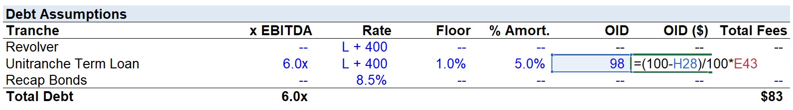
Original Issue Discount (OID)
You may have noticed two new columns referring to an OID, which stands for “Original Issue Discount.”
Imagine you ask a friend to lend you $10,000 at 10% over 3 years. Your friend refuses, so as a way to make it more attractive, you offer the following “How about instead, you just give me $9,800, but when I pay you back, you’ll get $10,000, plus the 10% interest each year on the $10,000. That’s basically OID.
So when debt is issued at a discount to par value (98 in this simple example), the borrower gets $0.98 for every dollar owed.
For OID accounting, the difference between the principal ($10,000) and the issuance amount ($9,800) is $200. This $200 must be amortized over the term of the debt and treated as non-cash interest. This is identical to financing fee accounting (i.e. increases amortization, reduces earnings before taxes, and is a non-cash add-back on the cash flow statement).
Returning to our LBO modeling test, we calculate the OID by taking the Unitranche Term Loan issued at (99 OID/100) x $2,070mm = $21mm.
Since financing fees and OID will be treated identically in our model, we can simply lump this $21mm into the total financing fees column on the far right.
The financing fees are calculated as the 2% Financing Fee Assumption x the $2,070mm unitranche debt principal. Together the OID and fees amount to $62mm.
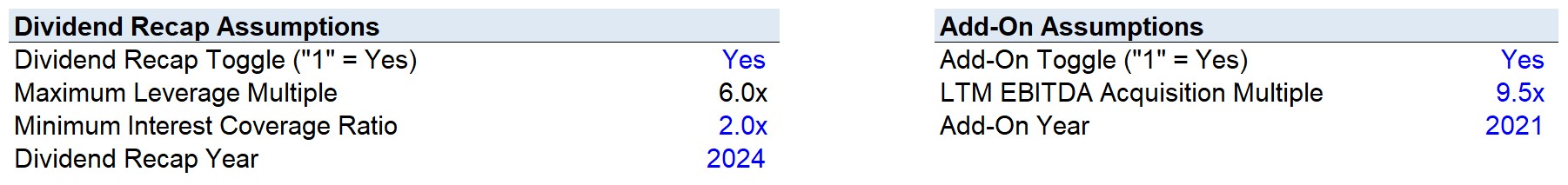
Dividend Recap Assumptions
To finish our assumptions section, we’ll list the dividend recap and add-on related assumptions.
Dividend recaps refer to when a sponsor raises debt to finance a dividend (i.e. akin to a home equity line). This is a common strategy to monetize an investment before a complete exit, and has the benefit of increasing the fund’s IRR from the earlier receipt of proceeds.
Completing a dividend recap is a risky action that should only be undertaken once the LBO has been, for lack of a better term, “validated” (i.e. proceeding better than originally anticipated) and the company has shown it can handle the additional lien.
Usually, recaps are done a few years after the initial acquisition – but there are some exceptions. For example, Bain’s dividend recap of BMC, which was covered in detail in our LBO course, is a real example of a private equity firm rapidly recovering some of its initial investment back.
Now, moving on to integrating a dividend recap into our model.
First, we will create a toggle for the dividend recap as we need the flexibility to not only choose the year but to switch it “Off”.
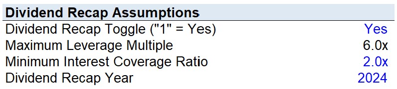
Here, we assume the lender provided two maintenance covenants and one additional restriction that JoeCo must abide by:
- Leverage Multiple: (Total Debt/EBITDA) must remain below 6.0x in all years and a dividend recap cannot be completed if the additional debt raises the leverage multiple above this threshold.
- Interest Coverage Ratio: (EBITDA/Interest Expense) must stay above 2.0x
- Timing Restrictions: The dividend recap cannot be done until two years have passed, therefore 2023 is the earliest the recap can be undertaken. We will create a toggle for the years the dividend recap can be done. Given the date-related covenants, we’ll create a drop-down list where the only options are restricted to N/A, 2023, 2024, and 2025. We’re going to assume the recap debt will be raised at the beginning of the “Recap Year,” so the recap debt is based on the prior year’s debt capacity, NOT the current period. Since the recap is completed at the beginning of the “Dividend Recap Year”, the full interest amount and mandatory amortization will be due.
As long as these two maintenance covenants and the timing restriction are followed, the sponsors are free to raise additional debt to pay themselves a dividend without having to refinance any debt.
Add-On Assumptions
Just as we did for the dividend recap, we will first list a toggle to have the option to switch it off.
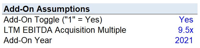
The “LTM EBITDA Acquisition Multiple” is assumed to be 9.5x and the lender has provided a $1,000mm revolver, i.e. the acquisition of TeaCo, if completed, is funded entirely by this revolver.
Lastly, we’ll include a drop-down list for the year the add-on is completed. Unlike the dividend recap, the add-on can be completed in any given year.
Step 2. Sources and Uses Table
We will now complete the Sources & Uses table. If you’ve gone through the Standard LBO modeling test, the structure should be familiar, but there are some distinctions:
- This transaction is NOT completed on a CFDF basis.
- There are TWO financial sponsors involved this time.
- There is NO equity rollover.
The completed Sources and Uses schedule for this take-private transaction is shown below:
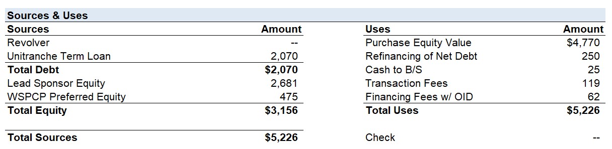
Note: The stated value of the unitranche loan is $2,070 million, which is NOT the actual dollar amount provided by the lender (i.e. recall the OID component). The offsetting factor is on the “Uses” side, in which the OID is embedded along with the financing fees. The OID causes the “Total Uses” to increase, meaning the sponsor equity contribution rises.
Uses Side
- Purchase Equity Value: We start on the Uses side with the “Purchase Equity Value”, which will be the $4,770mm entry equity value and NOT the entry enterprise value. The reason is the deal is a “take-private” and therefore not done on a cash-free, debt-free basis.
- Refinancing of Net Debt: Next, we have a new line item named “Refinancing of Net Debt”, which is equal to all the existing debt on JoeCo’s B/S minus its entire cash balance. The rationale is the acquired cash can be used to help with refinancing JoeCo’s debt at any given moment. This comes out to $250mm in debt that needs to be refinanced.
- Cash to B/S: Right below this line item is the “Cash to B/S”, which will ensure the minimum cash balance does not dip below $25mm since right above we used the entire cash balance in the formula for the net debt refinancing. Alternatively, we could have modeled it as “Excess Cash on B/S” on the “Sources” side, which is calculated by subtracting the Cash to B/S from the total cash balance. Then on the “Uses” side, there would be a line item for “Refinancing of Existing Debt” that just links to the total existing debt.
- Transaction and Financing Fees: The final two “Uses” are the “Transaction Fees” and “Financing Fees”. The financing fees of $62mm can just be linked to the calculation in the debt assumptions table. And the transaction fees are calculated as 2.5% of the offer value, which comes out to $119mm in advisory fees paid to the investment banks, consultants, accountants, etc. that helped complete this deal.
Sources Side
On the “Sources” side, we’ll start by listing the sources of debt capital, since the equity required is a function of the amount of debt raised.
- Revolver: Left undrawn at purchase
- Unitranche: $2,070mm was raised via the unitranche term loan, with the OID adjusted for in the “Uses” section.
- Equity: WSPCP invested $475mm of preferred equity, and the remaining equity required was “plugged” by the Lead Sponsor.
The equity invested by WSPCP is on a convertible preferred basis, which means the preferred shares include the option for WSPCP to convert the shares into a fixed number of common shares.
In effect, WSPCP receives either:
- Option 1: The “Accrued Value” of the investment at the 8.5% PIK rate – which has the benefit of downside protection via the PIK debt-like feature
- Option 2: The “Conversion Value” to common shares at the strike price of $1.25 – this provides WSPCP the option to participate in the potential upside of the common equity
This is a great place to mention the disconnect between equity and debt investors in the context of a dividend recap. The lender does not have the option to participate in the upside regardless of how well JoeCo performs. For the revolver and unitranche term loan, the maximum the institutional lender could earn is the interest payments and original principal repayment.
If the sponsors decide to proceed with a dividend recap, they are de-risking their investment, since some of their initial investment is retrieved before the exit. From the perspective of the lender, the bankruptcy risk of the borrower has just increased from the additional lien on the company.
Hence, in real life, debt covenants are significantly more restrictive and would typically include provisions that some (or all) of the existing debt must be refinanced before a dividend recap could be completed.
Note: This is the reason we intentionally had only one lender involved in the financing of this LBO – this lender pre-approved these plans, and the new debt raised is coming from them.
Step 3. Purchase Price Allocation (PPA)
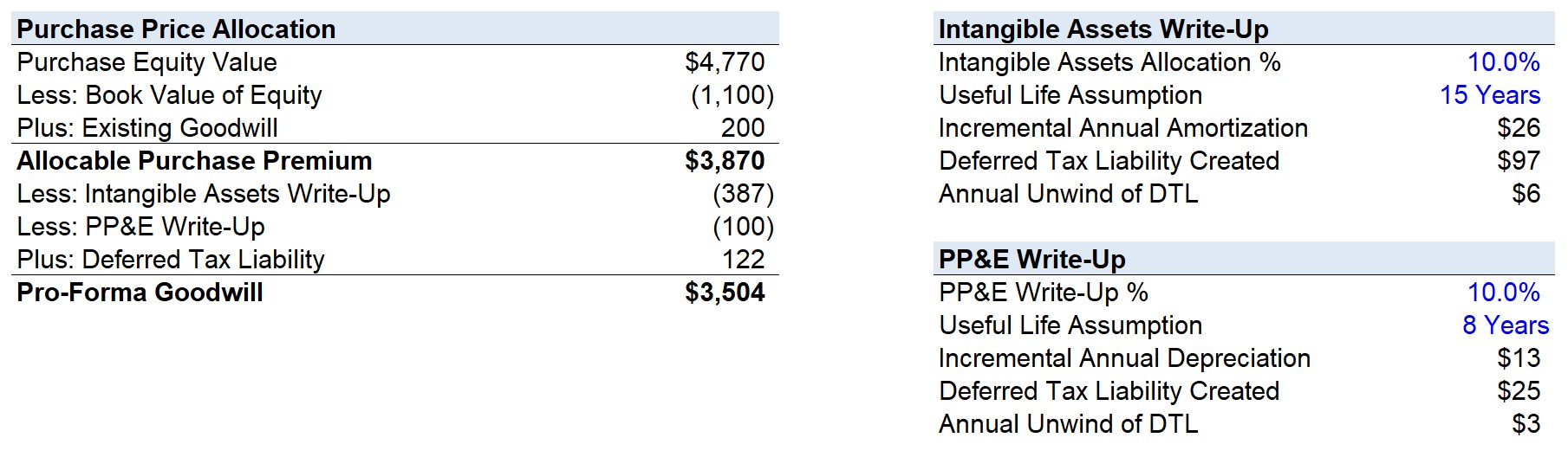
Next, we will go through the process of purchase price allocation:
As we noted earlier, we are not going through this step to forecast the 3-statements as we did in the Standard LBO Model Test. Instead, we are completing the PPA to calculate the values of the PP&E and Intangible Asset Write-Ups, the Incremental Amortization/Depreciation, and the Un-Wind of Deferred Tax Liabilities (“DTLs”).
All of these items must be calculated because they are reflected in the I/S and impact the free cash flow build that determines the amount of cash available to pay down debt.
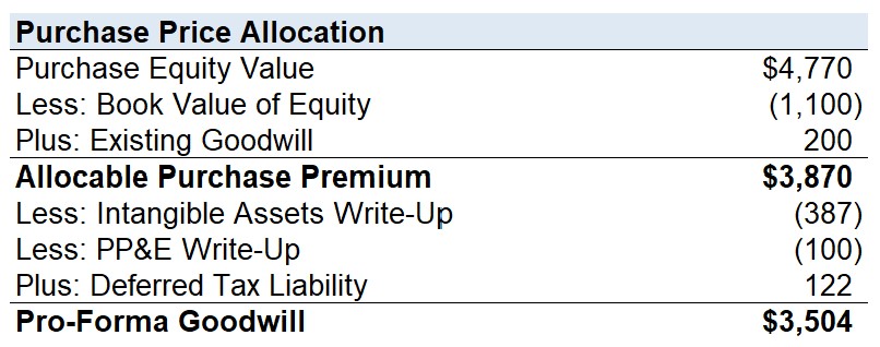
To get started, we will first link the purchase equity value from the transaction assumptions and subtract the book value of equity and existing goodwill to arrive at the “Allocable Purchase Premium” of $3,870mm – this is the excess paid that will flow towards goodwill once adjusted for write-ups/write-downs and DTLs.
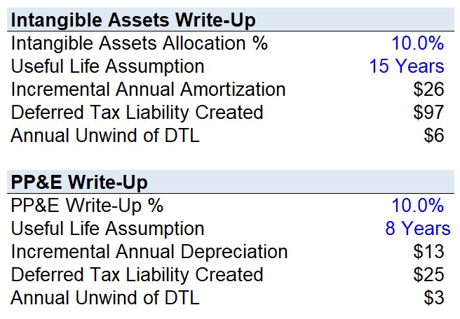
As the prompt mentioned, intangible assets were written up 10% with a useful life assumption of 15 years. This amounts to an “Intangible Assets Write-Up” of $387mm and an “Incremental Annual Amortization” of $26mm. We must not forget the DTL created, which will be $97mm and will be un-winded by $6mm each year.
Now for the PP&E write-up, the write-up was 10% of the LTM PP&E balance of $1,000mm to $1,100mm. As you can see, the “PP&E Write-Up” amounts to $100mm and the “Incremental Annual Depreciation” will be $13mm. The associated DTL created is $25mm and the annual unwind will be $3mm each year.
With the intangible assets and PP&E write-up sections completed, we can now calculate how much goodwill was created in this LBO. As we can see below, the total goodwill created was $3,504mm.
Step 4. Closing B/S Adjustments
With the PPA complete, we will now put together the Closing B/S – which is not necessary for this particular LBO modeling test but should still serve as good practice. It takes no more than a few minutes to complete, and it is an opportunity to check your work.
Unlike our Standard LBO where we build out a full 3-statement model – you do not get many chances to check your work, so you may find this beneficial even if it is not necessary.
For example, suppose that you mistakenly double-counted the Cash to B/S in the Sources & Uses table. The ending balance sheet would not balance, and you’d fix your mistake immediately.
While we do technically have a “Check” for the Sources & Uses table, it is frankly not that useful, because there is an equity “plug” that makes the two sides balance. In fact, you’d have to make an absurd mistake in the S&U schedule for it not to balance.
Assets Side
- Goodwill: The calculated pro-forma goodwill is $3,504mm and flows into the Closing B/S, and the existing goodwill is wiped out to prevent double-counting.
- Cash to B/S: For the rest of the assets side, Cash to B/S is a positive debit of $25mm, and the existing cash balance is wiped out. But rather than being wiped out to go to the seller as it would in a CFDF deal, the amount was used for the refinancing of the existing pre-LBO debt.
- PP&E Write-Up and Intangible Assets: We also see the $100mm write-up of PP&E and the closing intangible assets balance of $387mm as we calculated in the PPA.
Liabilities and Equity Side
- Pre-LBO Debt: On the liabilities side, we see the existing capital structure was completely wiped out, and the “Sources” side was brought into the closing B/S. The pre-LBO debt of $450mm was wiped out, while the new debt tranches raised are inputted as credits.
- Capitalized Financing Fee + OID: The capitalized financing fee, which includes the OID, is shown as a debit of $62mm and the “Deferred Tax Liability” of $122mm is shown on the credits side.
- Book Value of Equity: Finally, the existing book value of equity of $1,100mm is wiped out alongside the extra deduction of the transaction fees on the debits side, and then the new equity investment of $3,177mm will flow into the credits side.
Step 5. Add-On Financial Build
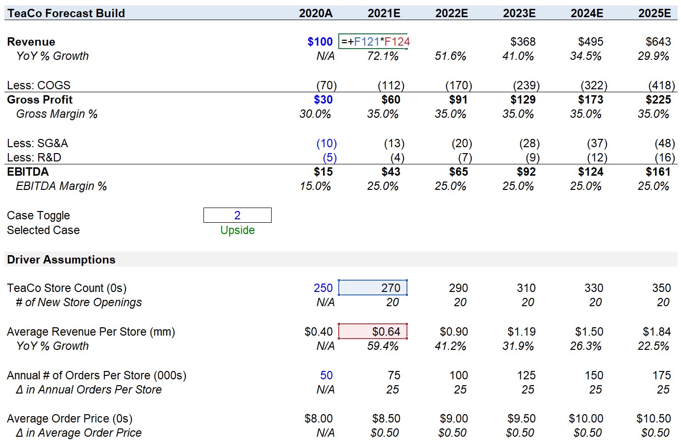
Our end goal for this step is to get the following pro-forma financials for TeaCo:
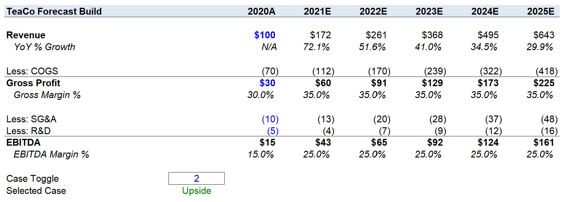
Notice the case toggle right above, which we created to easily switch between the three operating scenarios for the Add-On’s revenue and EBITDA forecasts:
- Base Case: The base case represents the conservative forecast that is most probable to occur. The assumptions used should be reasonable and in line with past historical performance. As a general proxy, if you calculate the average historical growth rates and margins of the company, the outputs should be close to what is projected. The exception would be if this were a turnaround deal, in which the past performance would not reflect future expectations.
- Upside Case: The upside case tends to be close to management guidance. Management projections usually contain some optimism (and they rightfully should). But one factor to consider when assessing management assumptions is the potential for an earn-out as part of the transaction. An earn-out is used to bridge the gap between valuation differences between the buyer and seller and is a contingency payment based on reaching an EBITDA (or Revenue) target.
- Downside Case: The downside case reflects how a business should perform during an economic downturn. The severity of the impact and how much the performance deviates from the Base Case depends on the industry the company operates. Hence, PE investors pursue investment opportunities in non-cyclical industries. If you switch our “Case Toggle” to “3”, the Downside Case is shown, and you’ll see how the revenue declines in the forecast and the margin contraction. In this case, we expect the downside case is actually not too bad because of the non-cyclicality of this add-on.
Note: The downside case in an LBO model often reflects “disappointing” financial results, rather than the company’s performance under a recession. In these situations, there will be another case specifically named the “Recessionary Case”.
Earn-Outs in LBOs
In nearly all cases, a seller and a sell-side representative have the incentive to sell at the highest valuation. However, if a private equity firm has a history (i.e. reputation) of structuring deals with earn-outs, the sell-side advisor may suggest to the seller to be more conservative.
Earn-outs are based on hitting target figures, and if the management pitches unrealistic numbers – they have effectively shot themselves in the foot because the targets used are the ones that came out of their mouths. In these scenarios, the deal would either not close, or the management would accept a lower valuation and upfront payment.
Revenue Build of TeaCo (Add-On Acquisition)
So now that we know where we’re trying to go, how do we get there?
We need to create a revenue build for TeaCo that reflects the unit economics provided in the Prompt.
To forecast the revenue of TeaCo, we have first broken the business down to some of its most basic unit economics:
In terms of TeaCo’s revenue drivers, the basic idea is that revenue is a function of: “Average Revenue per Store ($)” × “# of Stores”.
The other key driver is, “Average Revenue Per Store”, which is calculated using the formula below.
- Average Revenue Per Store = Average Order Price ($)” × “# of Orders per Store
Using this logic, our “Average Revenue Per Store” is approximately ~$400k in 2020.
Quick Reminder
Be careful of the units used – as you can see in our model, we explicitly wrote out the units used for each to ensure the reviewer is aware of what units we are using.
The “Average Order Price” was the underlying driver that we were working our way down to. The order price or average selling price (i.e. “ASP”) is usually the minimum level of specificity an LBO Model Test will need you to have.
The purpose of doing this is: you want specific figures to reference (i.e. the average order price increased $X amount and the number of new stores opened was X, rather than revenue will grow X% just because it seems reasonable).
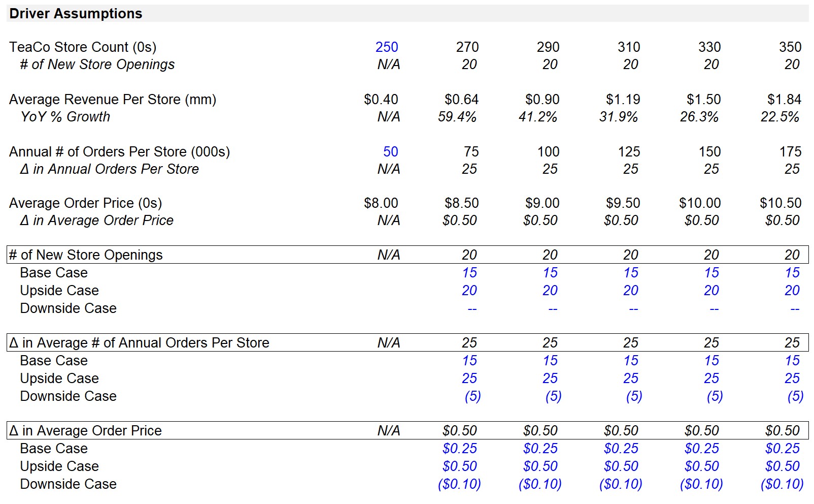
Using those figures, we can build out our case functionalities. The following three assumptions serve as our model’s revenue drivers:
- # of New Store Openings
- Δ in Annual Orders Per Store
- Δ in Average Order Price
We will make assumptions for how these three variables will differ under the three cases, and this will ultimately drive our revenue for the year.
The three revenue drivers we will forecast across the three case assumptions are shown below:
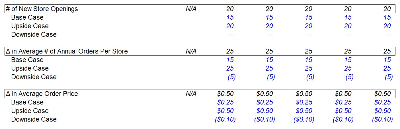
The “OFFSET” function will pick the case selected based on the toggle. For example, the picture above is reflecting the “Upside Case” of TeaCo.
The next step is to work our way up to the total revenue each year forecast. We will begin with the “Average Revenue Per Store”, which will be a function of our “Average Annual Order Count” and “Average Order Price” assumptions – just be sure to divide the store count by 1,000 before multiplying the two.
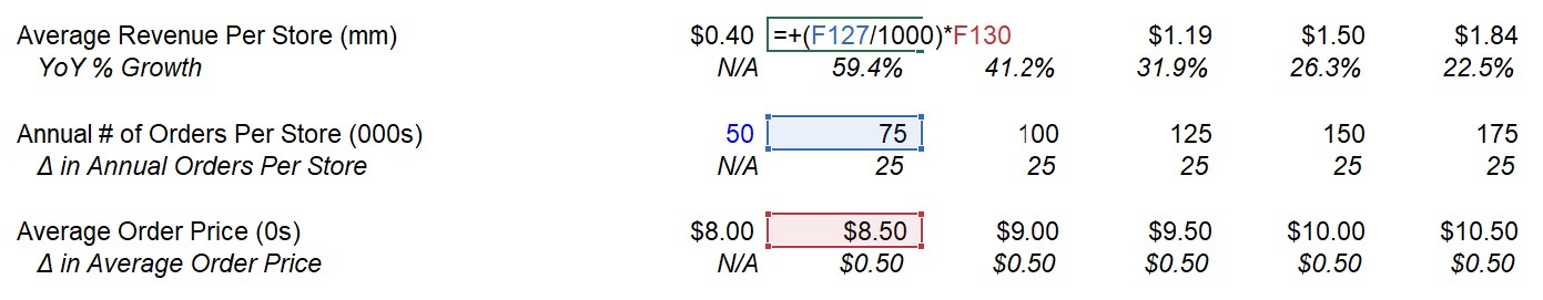
The “Δ in Annual Orders Per Store” and “Δ in Average Order Price” were pulled from the assumptions table, and will impact the unit driver it is connected to. For example, the $0.50 increase in average order price and the 25 new stores opened brings the number of stores in 2021 to 75.
This ultimately drives the “Average Revenue Per Store”, which we did not forecast individually, as mentioned earlier. We want to identify the unit economics that determines the average revenue per store, instead of creating a forecast without actual figures to reference.
For example, on the job, you would want to be able to say: “TeaCo needs to open X number of new stores and increase its average order price by $X”.
Then, we will multiply the “Average Revenue Per Store” by the “TeaCo Store Count”, which is driven by our assumption of the number of new stores opened each year. Doing so will give the total revenue of TeaCo for each year.
To finish our forecast, we created three case functionalities for the Gross Margin %, SG&A % of Revenue, and R&D % of Revenue, and integrated them into our forecast.
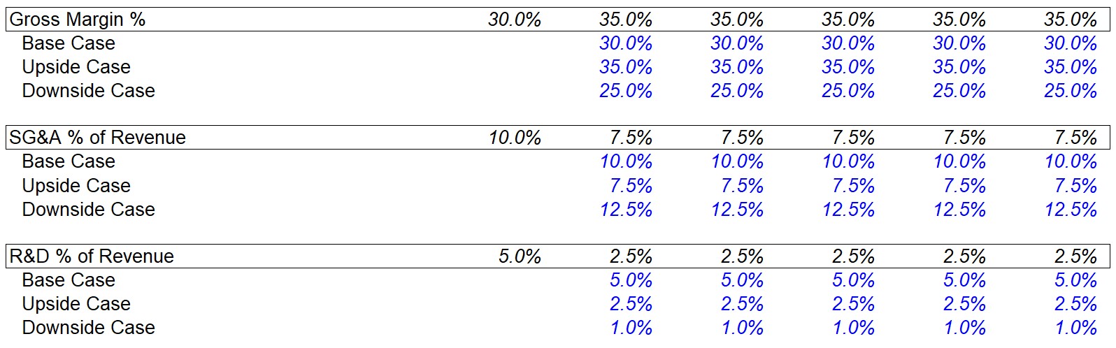
For most LBO model tests, this is perfectly fine to do, and you will actually not have enough details to do a full expense build usually.
Given the time constraint, at most you might need to create some type of simple forecast based on employee count, and then back into the annual salaries if the figures are provided, or do what we just did above for individual segments.
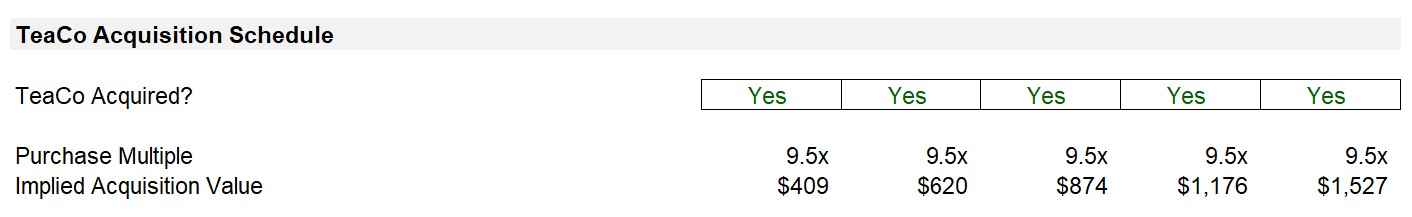
Based on the completed forecast of TeaCo, we can establish the company is currently in the growth stage of its maturity cycle, and therefore it might be best for JoeCo to complete the add-on as early as possible before the purchase price would exceed $500mm.
Lastly, we tracked our add-on acquisition and the implied purchase price in the schedule below:
Step 6. Pro Forma Financial Forecast
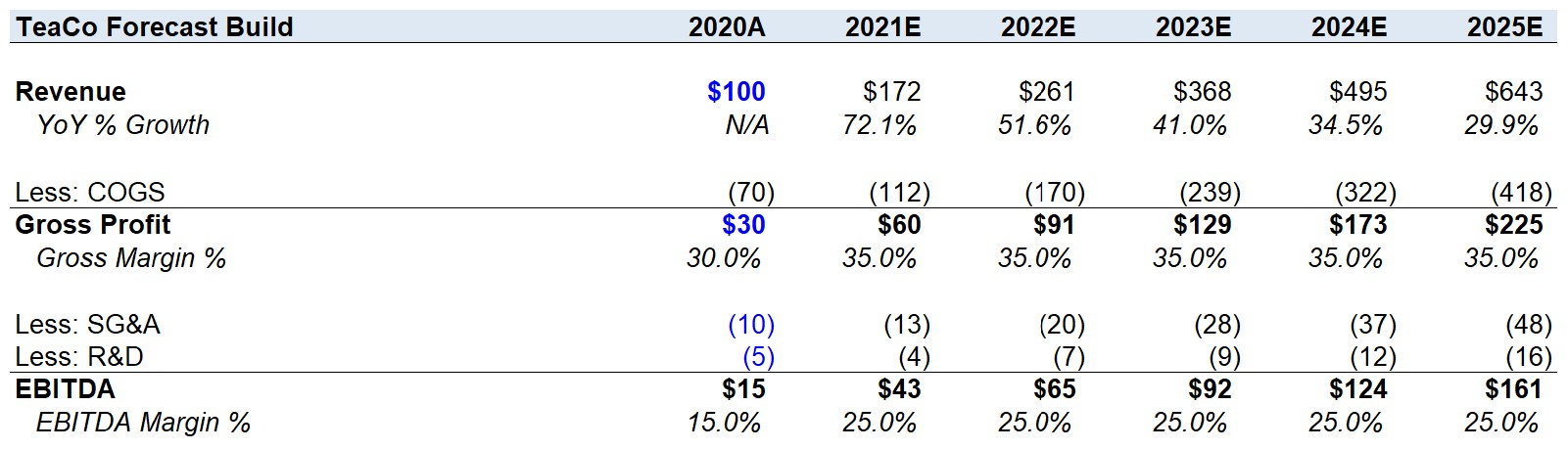
Pro Forma Income Statement
With TeaCo’s financial build complete, we’ll now forecast JoeCo’s financials.
Our goal in this section is to forecast the income statement and construct the free cash flow build.
JoeCo Standalone Operating Forecast
In the section beneath the financial forecast, we’ll place the assumptions driving JoeCo’s forecast. Per usual, we’ll have these assumptions placed below the summary financial forecast as a general modeling best practice.
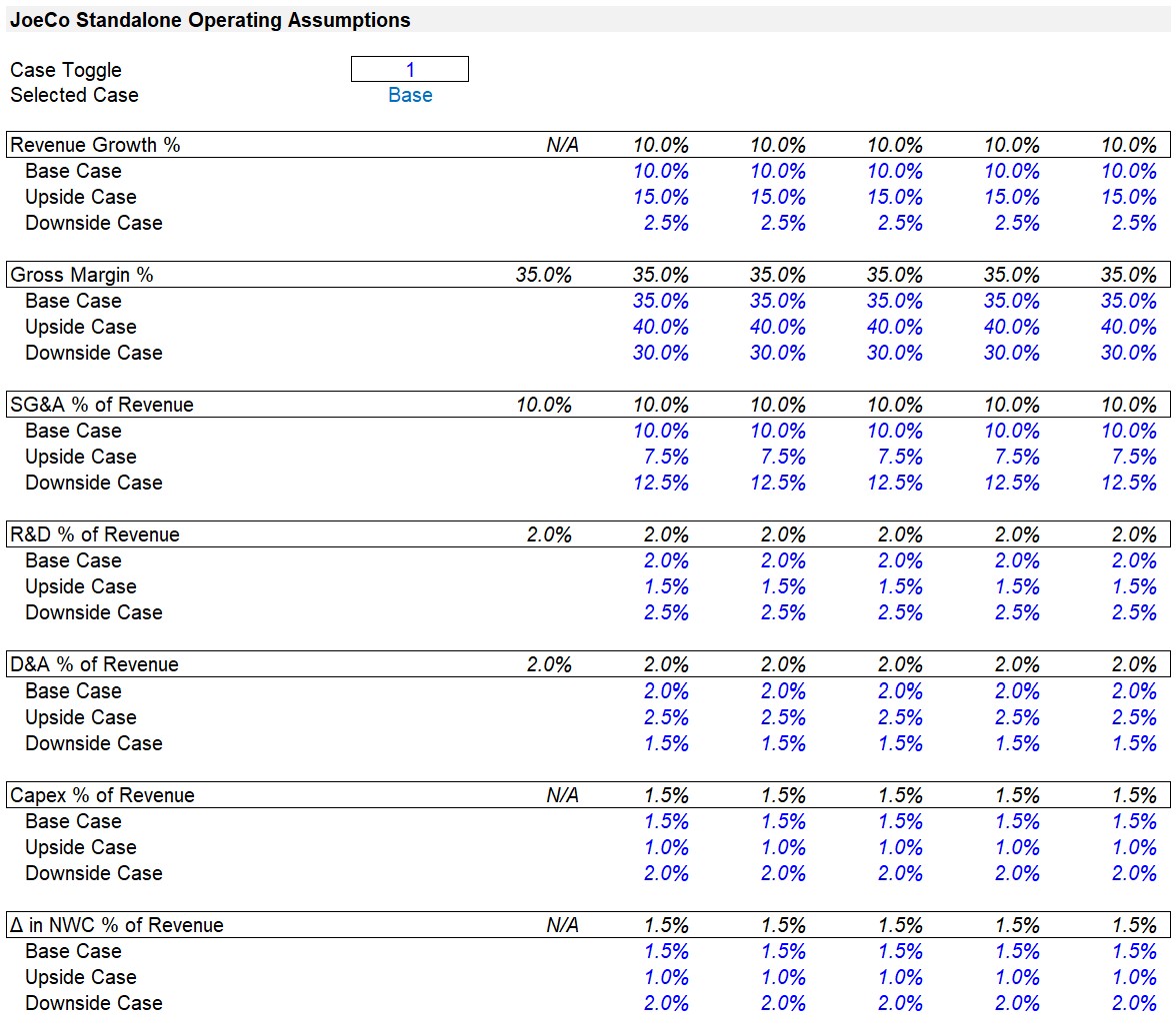
Note that the operating case toggle should be separate from the one used for TeaCo as we want the flexibility to view the two companies under separate assumptions.
For example, if JoeCo is performing in line with its upside side, it may lead sponsors to question whether to continue doing what is working and reinvest more into JoeCo, particularly if TeaCo has been underperforming.
This is also the reason we have separate line items for the pro forma consolidated financials. We can view the impact of TeaCo by switching the toggle “ON”/”OFF” and viewing the changes in the pro forma growth rates and margin profile.
Since you’ve already gone through how to do a revenue buildup for TeacCo, for JoeCo, we use a simple, % revenue growth approach for JoeCo in the interest of time. In addition, we also include baseline, upside, and downside assumptions for JoeCo’s operating expenses, as well as changes in NWC (which will be used later to forecast cash flows):
TeaCo Add-On Integration
Integrating TeaCo’s financials into the model will use the toggle switch we created earlier. All of TeaCo’s line items will use an “IF (AND(“ function to confirm:
- The “Add-On Toggle” is switched to “Yes”
- The “TeaCo Acquired?” line item states “Yes”
If both are “Yes”, then TeaCo outputs will be added to JoeCo’s financials:
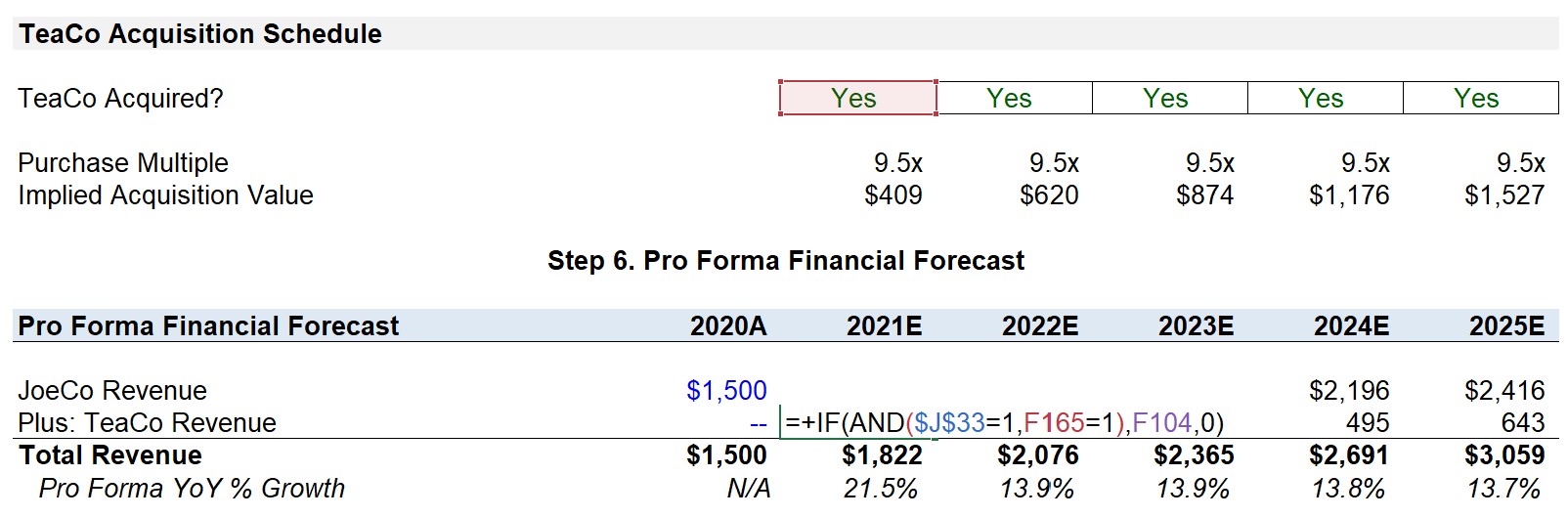
We follow the same approach for COGS, SG&A, and R&D to arrive at EBITDA.
Management Earn-Out
For the management earn-out, we’ll leave the line blank for now, as we will return to it shortly. We calculate this separately (even though this is an SG&A expense), to avoid a circularity, since the earn-out itself is based on EBITDA.
EBITDA → EBIT
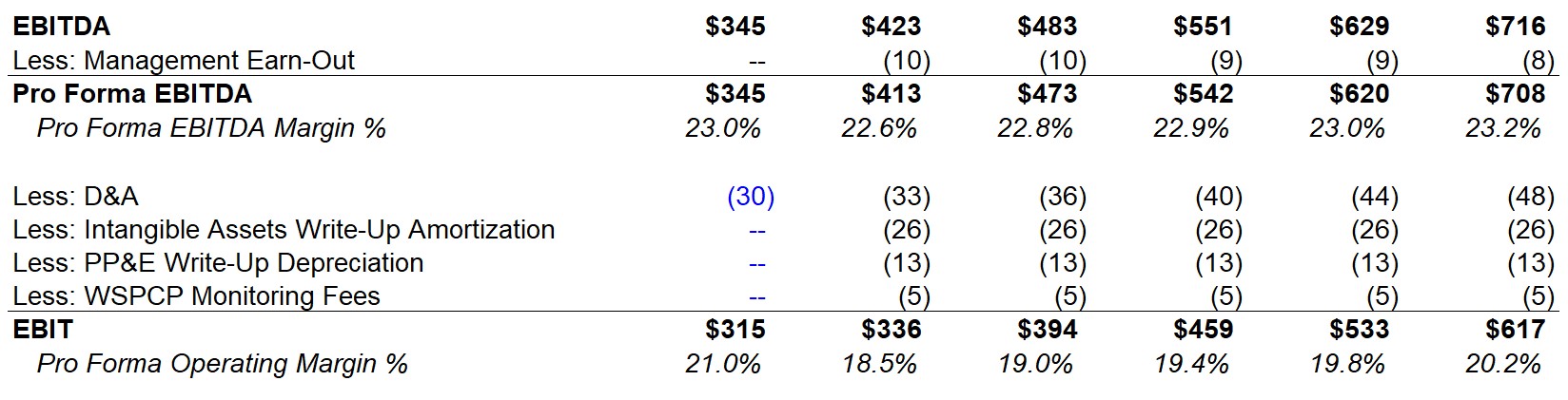
Now that we have the calculations for the EBITDA set, we will subtract “D&A”, the “Intangible Assets Write-Up Amortization”, “PP&E Write-Up Depreciation”, and the “WSPCP Monitoring Fees”.
This should be very straightforward – the D&A is projected as a percentage of revenue while the incremental amortization and depreciation write-ups are pulled straight from the PPA schedule, and the WSPCP monitoring fees were listed in the assumptions section as $5mm each year.
Interest Expense and Amortization of Financing Fees + OID
While the interest expense cannot yet be calculated since we have not built the debt schedule, the amortization of the financing fees and OID can be calculated by dividing the $62mm in total financing fees by the financing fees amortization period of 8 years to get a value of $8mm.
We will also need to return to this section later to reflect interest and fees from recap debt.
From there, once we subtract taxes based on the 25% tax rate assumption, we have arrived at net income, the “bottom line.”
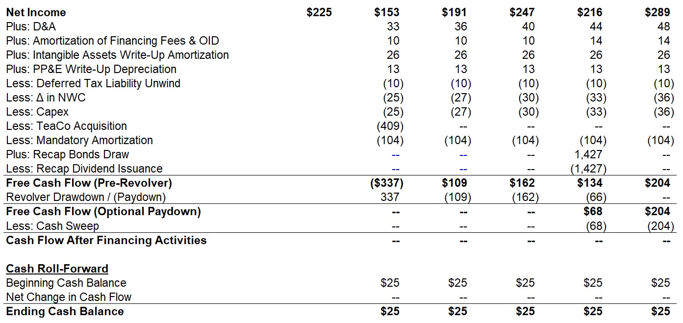
Free Cash Flow Forecast
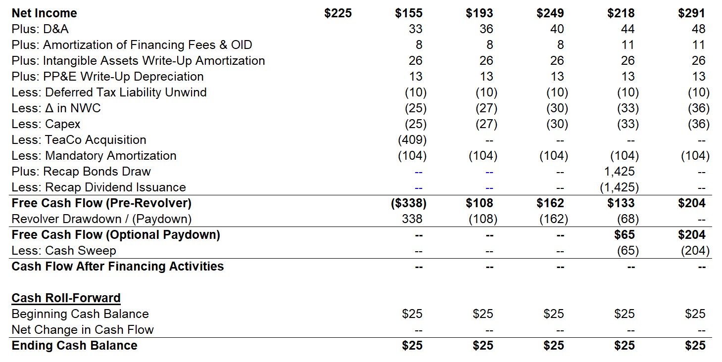
We can now construct our free cash flow build. Although we don’t break up the cash flow statement formally into the 3 sections (operations, investing, and financing), you’ll see that they’re all there.
1) Cash from Operations
- Add back all the non-cash expenses such as “D&A”, “Amortization of Financing Fees & OID”, “PIK Interest”, “Intangible Assets Write-Up Amortization”, and “PP&E Write-Up Depreciation”
- Deduct the “Deferred Tax Liability Unwind” and “Δ in NWC.”
2) Cash from Investing
- The usual cash outflow, Capex, will first be accounted for
- Reflect the cash consideration paid for the TeaCo add-on using a similar “IF(AND(” function used earlier:

3) Cash from Financing
- While we haven’t built the debt schedule yet, in this area we will eventually subtract the “Mandatory Unitranche Term Loan Amortization”
- There are two new line items below, the “Recap Debt Draw”, and “Recap Dividend Issuance” that we will also leave blank for now
- The remaining line items such as the “Revolver Drawdown/(Paydown)”, “Free Cash Flow Available (Optional Paydown)”, “Cash Sweep”, “Cash Flow After Financing Activities”, and the Cash Roll-Forward cannot be filled out at this point since the debt schedule has not been completed.
The result is Free Cash Flow (Pre-Revolver):
Step 7. Management Contingency Payments
Before we turn to the Debt Schedule, let’s calculate the earn-out that we left off the income statement earlier.
Each year, the management team has the potential to receive up to $10mm in additional compensation if all three threshold levels are met.
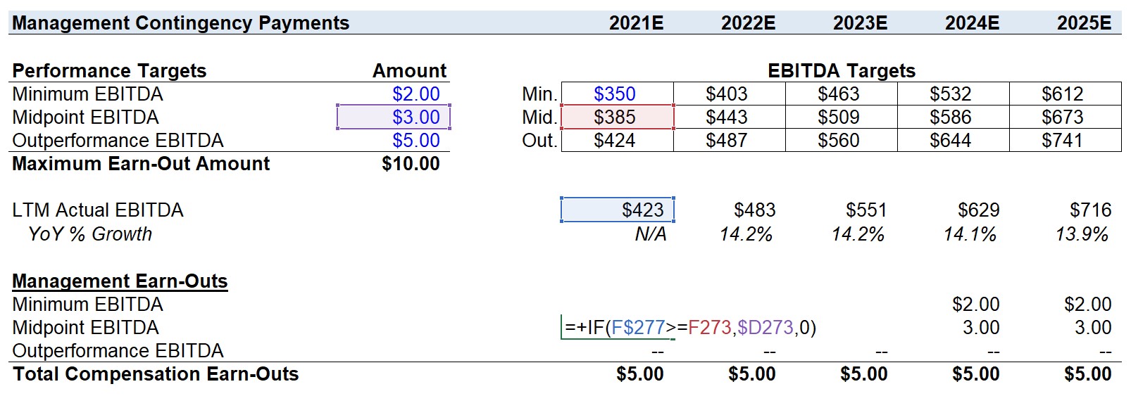
If the “Minimum EBITDA” hurdle is met, $2mm is earned, meeting the “Midpoint EBITDA” is an additional $3mm, and “Outperformance EBITDA” results in $5mm to total $10mm as the maximum earn-out in a given year. We can set this up as follows:
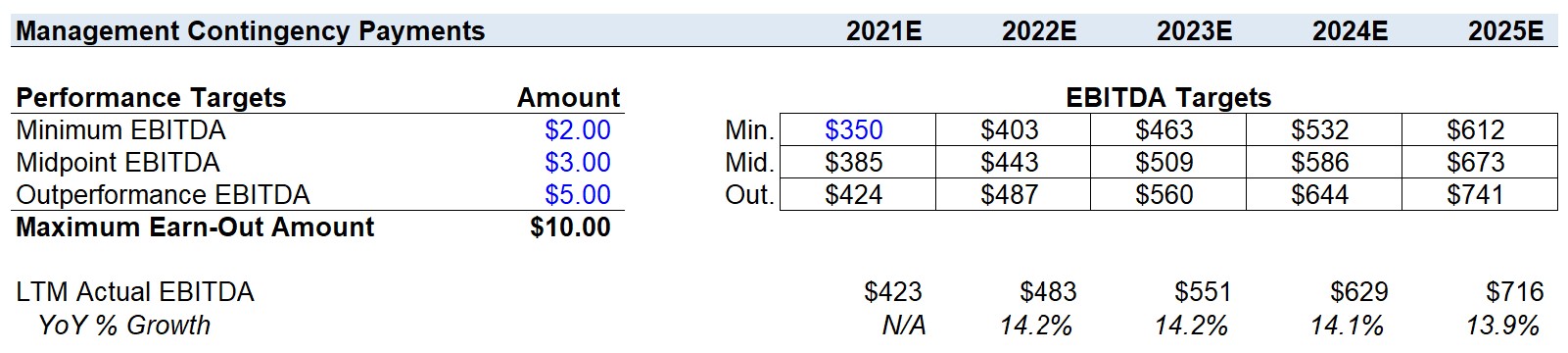
We then calculate the earn-outs based on the LTM forecast for EBITDA:
Next, we will calculate the pro-rata adjustments – which refer to how management may have missed a certain target, but the excess EBITDA over the threshold will be compensated in proportion to how close to reaching the next target the EBITDA was.
The “Excess EBITDA” calculation will use an “IF(AND(“ function with two logics.
- Confirm LTM EBITDA is greater than the previous target hurdle, meaning the next target was not met, but there is some excess EBITDA
- Confirm the target in question was indeed missed (i.e. equal to “0”)
If both logics are true, the actual LTM EBITDA will be deducted from the missed target EBITDA.
The “Excess Over Minimum” is shown:
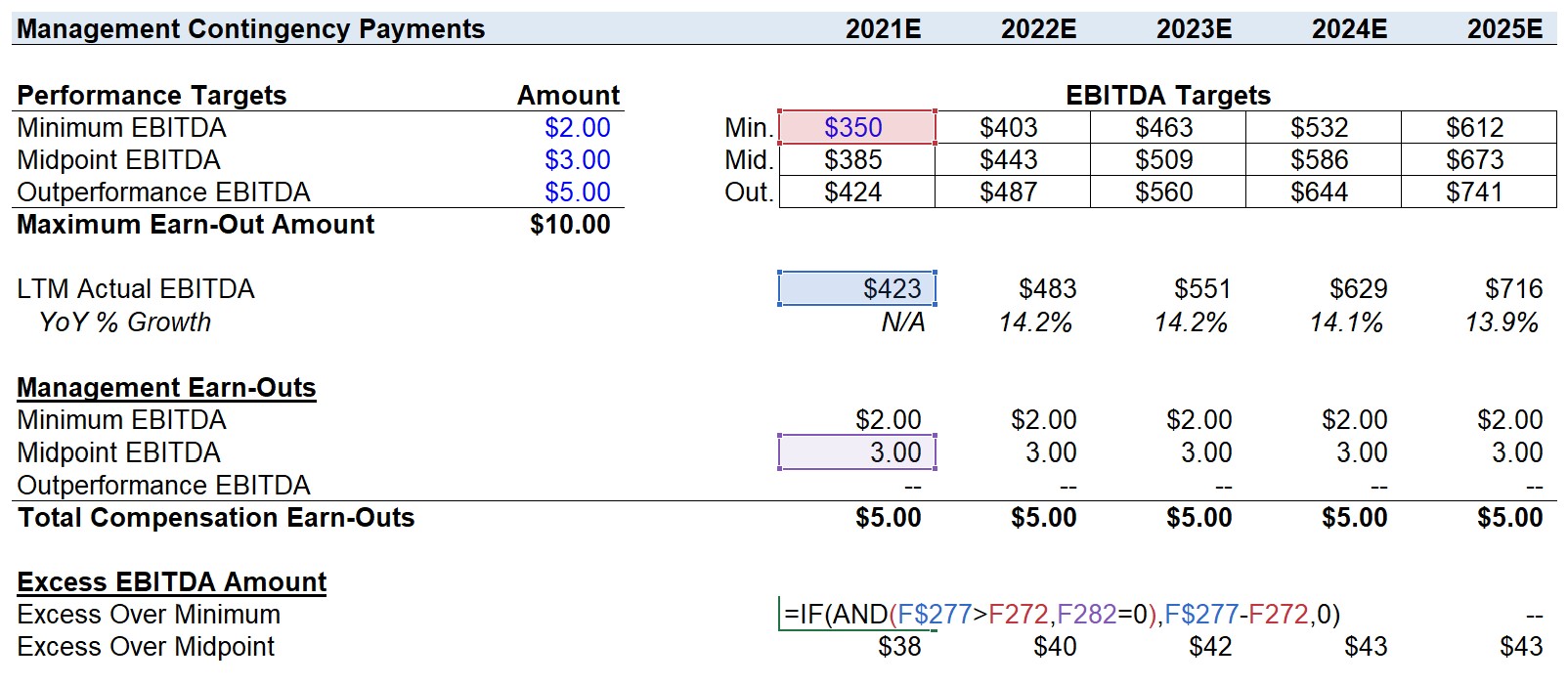
Note how in the examples shown above, the “Excess Over Minimum” is zero, because the “Midpoint EBITDA” target was met each period under this case selection, i.e. this is what the 2nd logic check ensures (i.e. the “F282=0” in the picture above).
Next, the “Excess Over Midpoint” is shown:
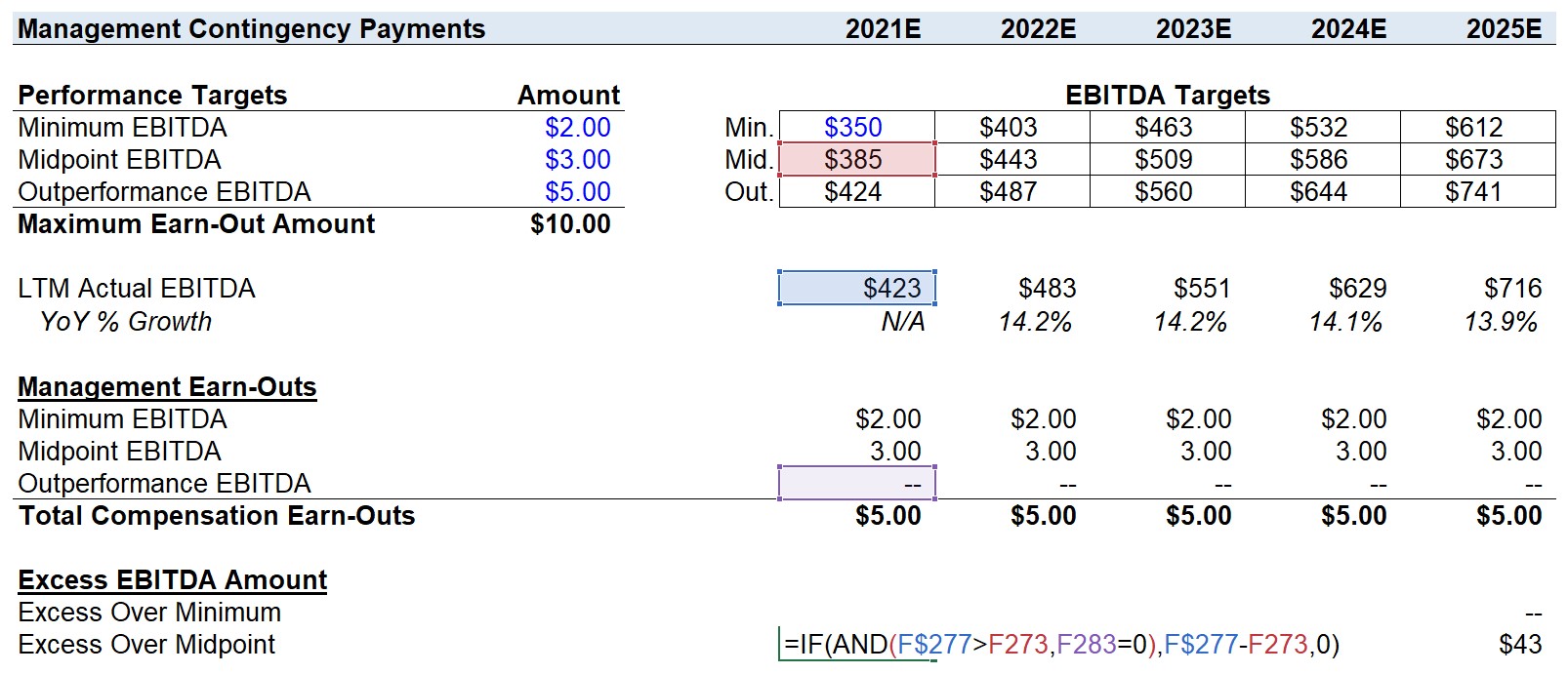
Thus, the only relevant pro-rata adjustment for 2021 is for the “Outperformance EBITDA”, in which the “Excess Over Midpoint” is $38mm. From a glance, we can see this is just ~$1mm short of meeting the target, so the pro-rata adjustment should bring the total bonus paid close to $10mm.
The formula for the “Midpoint EBITDA” pro-rata adjustment is shown below:
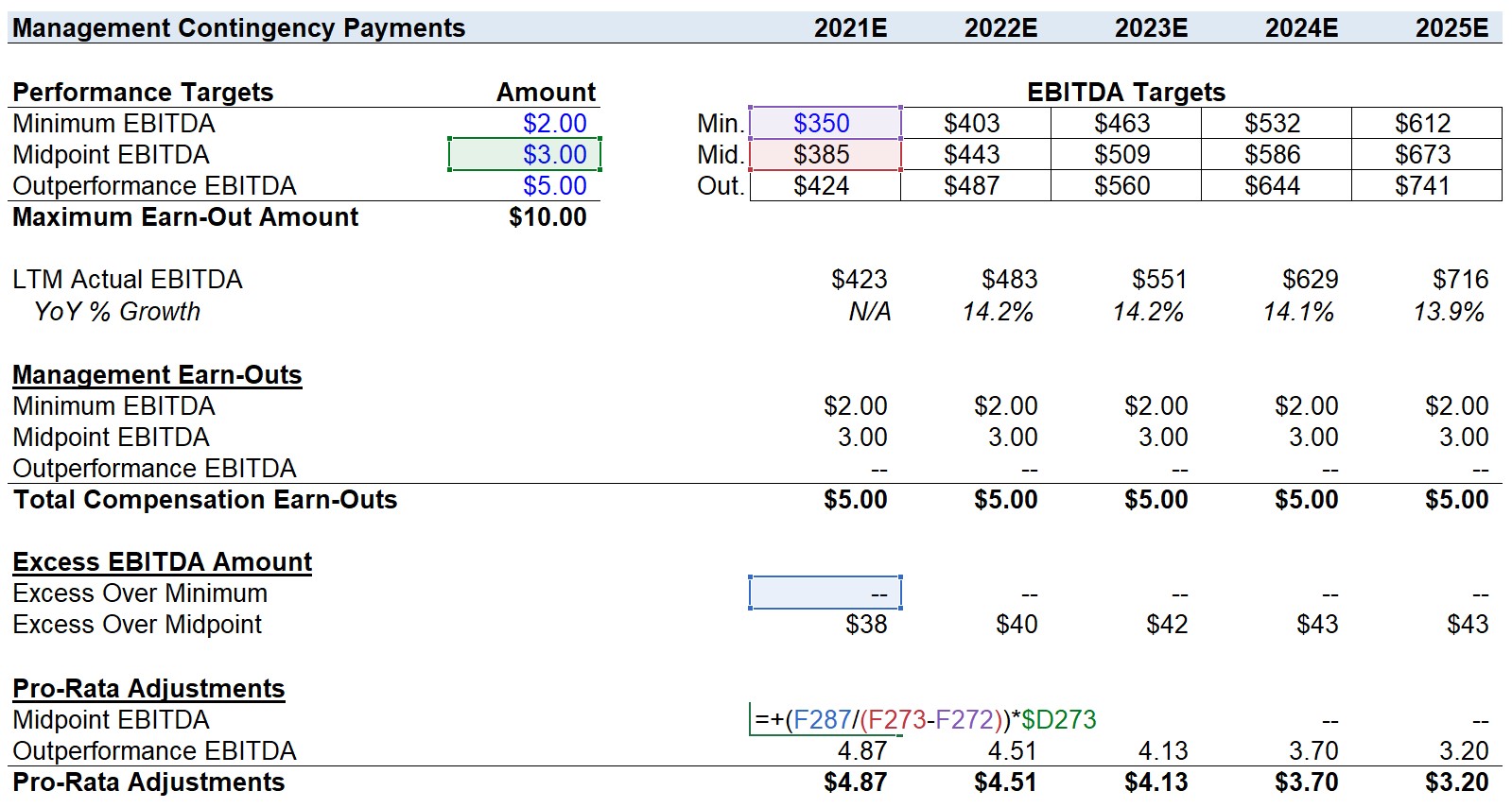
The “Excess Over Minimum” is zero each year because the “Midpoint EBITDA” was met, so the only pro-rata adjustments under this case selection will be for the “Outperformance EBITDA”.
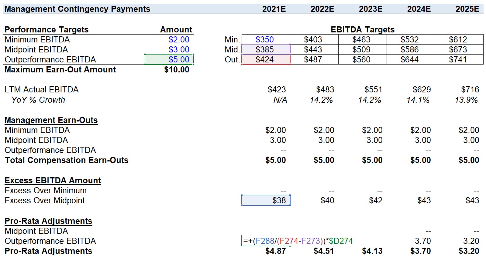
The pro-rata adjustment for the “Outperformance EBITDA” is shown below. As you can see, the formula takes the “Excess Over Midpoint” and divides it by the difference between the “Outperformance EBITDA” and “Midpoint EBITDA”. Then, this percentage will be multiplied by the “Outperformance EBITDA” proceed of $5.0mm.
For 2021, the “Outperformance EBITDA” pro-rata adjustment will be $4.87mm.
Below is the completed “Management Contingency Payments” table:
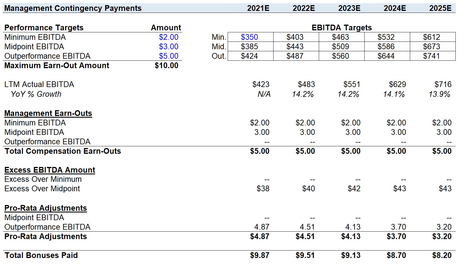
As we mentioned earlier, the “Outperformance EBITDA” target was just ~$1mm off, so as a sanity check this bonus amount in 2021 (i.e. the $9.87mm payout) seems reasonable.
The amount in bonuses paid will vary significantly by the assumptions used. For example, if you switch the JoeCo case selection to the “Downside Case”, not a penny is paid out to the management team in extra compensation because not even the minimum was met.
There are no pro-rata adjustments for almost meeting the “Minimum EBITDA”. For the first target, it is an “all or nothing” type arrangement.
This is the reason why there are only two pro-rata adjustments for almost hitting the “Midpoint EBITDA” and nearly reaching the “Outperformance EBITDA”.
On the flip side, any excess above the “Outperformance EBITDA” will NOT result in any extra compensation either. The maximum that can be earned is $10mm each year.
If the target is met each year, this is in no way a negative for the sponsors as it means that JoeCo is performing well.
In a sense, this type of compensation earn-out is an attempt to replicate management rollover equity, but there are still some limitations (i.e. rollover equity is preferable, given there is more for the management to lose than missing out on some bonus payments).
But to wrap this section up, the “Total Bonuses Paid” will be the sum of the “Total Compensation Earn-Outs” and the “Pro-Rata Adjustments”, which flows into the financial build before the “Pro-Forma EBITDA” line item.
Step 8. Debt Schedule
To finish our income statement and cash flow statement build, we must complete the debt schedule.
The first step will be to determine if there’s enough cash to pay down the revolver:
Then, we will see if there’s any excess cash remaining to sweep into the unitranche debt:
And finally, we can determine if there’s excess debt capacity to fund a dividend recap:
Going further into the optional repayments, we reference “Free Cash Flow (Pre-Revolver)” on the CFS into the Debt Schedule and rename the line item “Excess Cash Available for Revolver.” We want to see this number without having to constantly scroll back up to the CFS.
Keep in mind that this line is post-mandatory amortization for all the debt tranches, and thus the “Excess” in the name. The only places this excess cash can go towards are:
- Paydown of Revolver
- Additional Prepayment of Unitranche
Since the prompt said no prepayment is allowed for Recap Debt, we do not have to model a cash sweep for that.
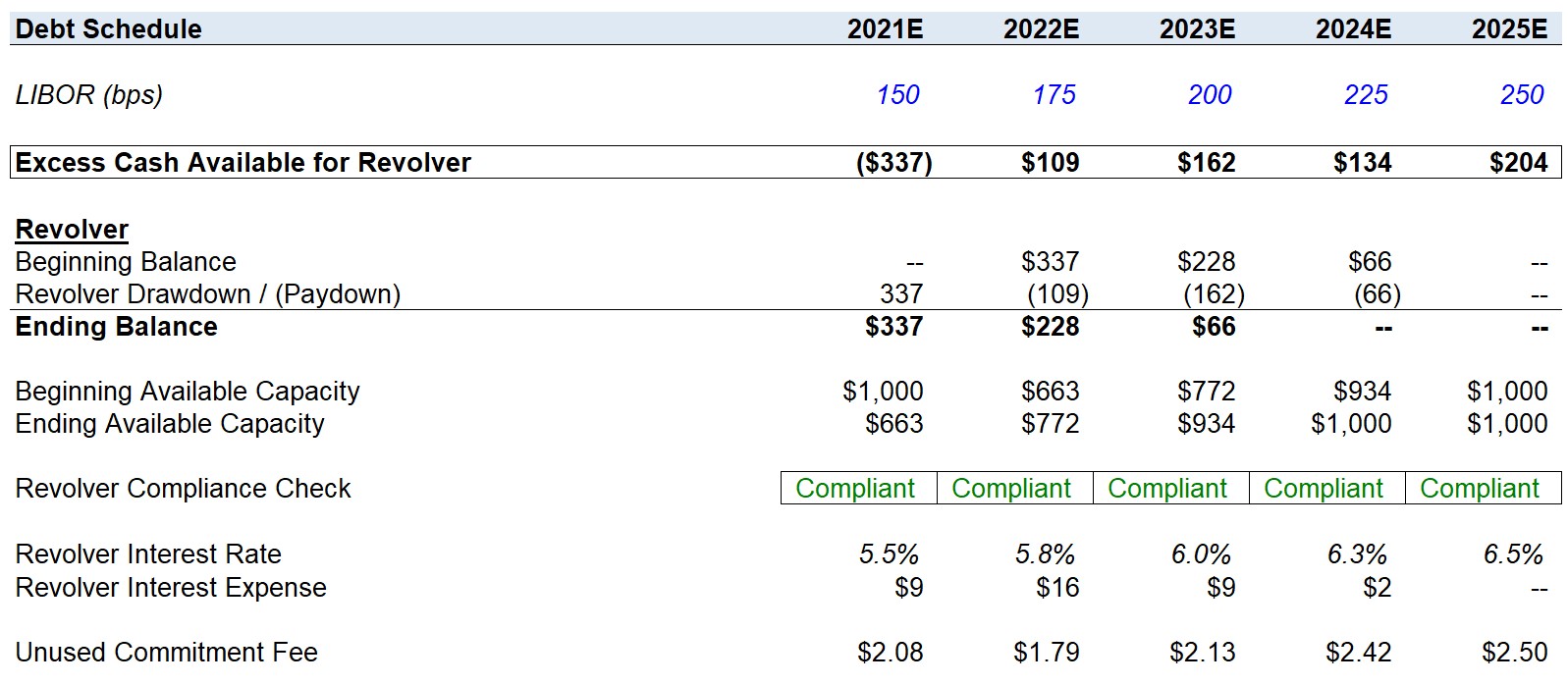
Revolver
The mechanics of the revolver are no different from the previous Standard LBO Modeling Test. The only notable difference is that the sponsors are given a much larger and fixed maximum capacity of $1,000 million:
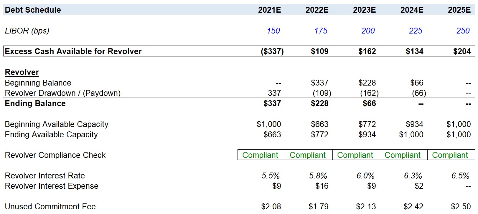
So how do we interpret what’s happening?
JoeCo paid $409mm to acquire TeaCo in 2021 and did not have sufficient cash to fund this acquisition using the free cash flows it generates alone. Thus, $337mm was drawn from the revolving credit line as intended.
While there is still significant flexibility for JoeCo to operate after the add-on, we included a “Revolver Compliance Check” that ensures the “Ending Available Capacity” never dips below zero.
Revolver Usage: LBO Modeling Tests vs. Reality
The usage of the revolver as an acquisition funding source contradicts many of our past articles, where we stated the revolver, in most cases, is meant to meet short-term working capital requirements and act as a “corporate credit card”.
But when it comes to modeling tests, it is actually quite common for this sort of assumption to be made, where an add-on or a significant capital expenditure is funded using a revolver.
After 2021, free cash flows turn positive and all go toward paying down the revolver given its seniority in the capital structure. By 2024, the revolver balance has been fully paid off and then we see the first cash sweep for the unitranche term loan.
In terms of the revolver’s pricing, it is the floating rate of “LIBOR + 400” as we are used to seeing and the unused commitment fee will be $2.5mm in the years the revolver is not used.
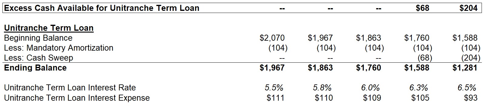
Unitranche Term Loan
Next in our debt waterfall, we have the unitranche term loan, which was structured with a mandatory amortization of 5% off the original face value amount each year, so the annual mandatory amortization is $104mm.
Now the question is whether there’s any excess cash to pay down the principal even further. Because the revolver gets paid down first, there’s only excess cash available in the last two years: Cash available to sweep into the Unitranche is calculated as the “Excess Cash Available for Revolver” plus the “Revolver Drawdown/(Paydown)” from the revolver roll-forward right above.
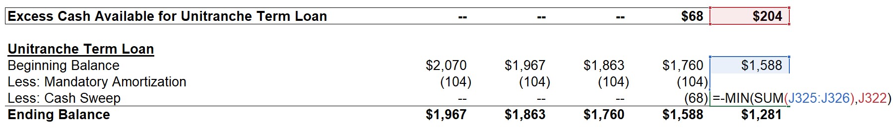
Since the principal balance cannot become a negative value, we also add a “MIN” function, such that the cash sweep formula is the minimum of:
- “SUM” of the Beginning Balance and Mandatory Amortization
- The “Excess Cash Available for Unitranche Term Loan”
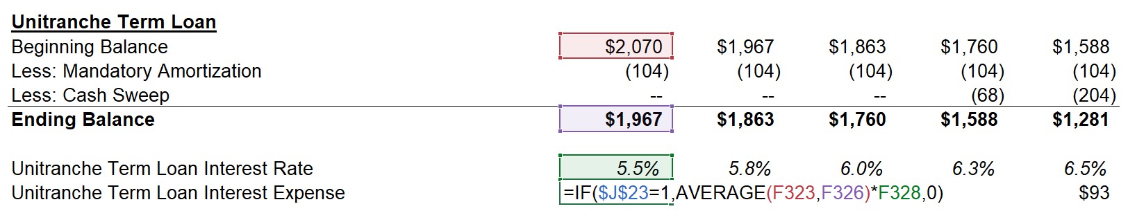
In terms of pricing, the unitranche term loan is priced at LIBOR + 400 with a 1% floor. Since LIBOR is above 100 basis points in the forecasted years, the floor actually has no impact on the interest rate pricing.
And as usual, the interest expense will be calculated off the beginning and ending balance of the term loan – which you can see does not actually reduce until the revolver is paid down as the cash sweep is delayed since the revolver comes first in the waterfall. But once the revolver balance returns to zero, we see the full cash sweep provision of the unitranche term loan in full effect.
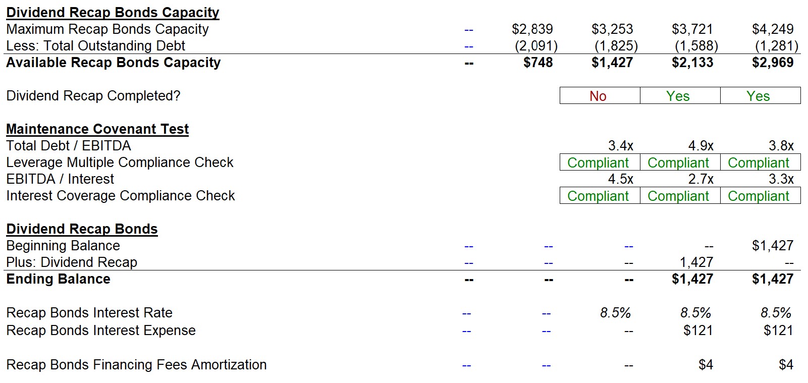
Dividend Recap Term Loan
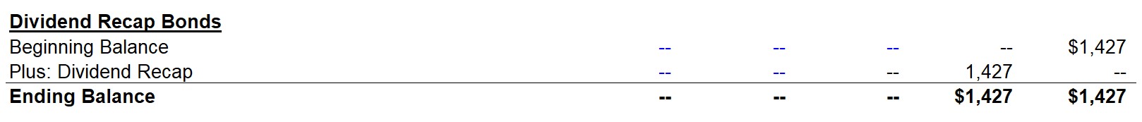
We will now cover the mechanics of the dividend recap, starting with the total available capacity that could be drawn to payout the one-time special dividend to equity shareholders. By the end, we’ll see that in 2024 that Sponsors can dividend recap $1.4 billion out of the company:
“Maximum Recap Debt Capacity” will be calculated by multiplying the EBITDA of the current year by the “Maximum Leverage Multiple” of 6.0x. And then, the total debt outstanding at the end of the same given period will be deducted from that amount.
To reiterate from earlier, as it bears repeating, the dividend recap is completed right at the beginning of the year. Thus, the actual recap drawdown links to the available debt capacity for the previous year.
For the example above, the $748mm is in the column for 2022. However, if a dividend recap were to be done in 2023, this would be the amount that could be drawn, as opposed to the $1,427mm.
In the “Available Recap Debt Capacity” line item, we include two additional logical functions to the formula:
- The “MAX” function is used to ensure the output is never below zero
- Confirms the “Recap Toggle” is equal to 1 (i.e. switched to “Yes”)
Debt Capacity Commentary
As EBITDA continues to grow and more debt is paid down via amortization and the cash sweep, the amount the sponsors can pay themselves increases.
The reason the available capacity is so low in 2023 relative to the other years is due to the acquisition of TeaCo, which was funded almost entirely by the revolver.
Recall, 6.0x is the initial leverage used during the transaction and we have a covenant in the lender agreement that we will not raise any additional debt to bring our leverage multiple above this level.
This is likely the reason why the Lead Sponsor said the most likely scenario would be a dividend recap in 2024 when the available capacity would be $1,427mm.
The Lead Sponsor here is attempting to balance de-risking their investment by receiving a portion of their initial capital back and paying themselves as large a dividend as possible.
In addition, an earlier dividend will have a more positive impact on IRR – which is the main marketing metric used when a firm is raising capital for its next fund.
Next, we will have a compliance check for the two maintenance covenants.
But to do this, we need to calculate the credit metrics the covenants are based on:
- Total Leverage Multiple = Total Debt/EBITDA
- Interest Coverage Ratio = EBITDA/Interest
When calculating the leverage multiple and coverage, use the figures for the current period.
The reason is that our “Available Recap Debt Capacity” already ensures the leverage multiple does not exceed 6.0x.
So if the sponsors completed a dividend recap in 2023, the amount that can be raised will be based on 2022, but the credit metrics we use for the compliance tests are the 2023 EOY numbers.
Because maintenance checks are completed on an annual basis typically at the end of the year, it would not make sense to look at the previous year’s credit metrics. It is the year the recap was completed and the forward-looking projections that matter to JoeCo and the lender.
Now moving on the roll forward for the dividend recap term loan. The “Plus: Dividend Recap” will use a simple “IF” function that confirms the “Recap Year” selected is equal to the current year, then the “Available Recap Debt Capacity” from the previous year will be output.
This represents the amount in recap debt that could be raised in the current year.
Below is the formula for the dividend recap draw for 2024:
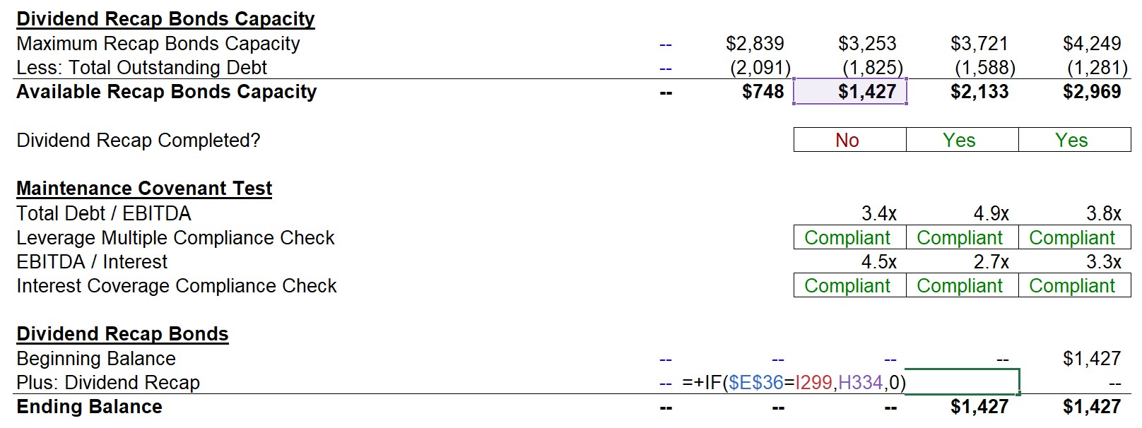
The maintenance covenant tests are in compliance, not just in 2024 but in 2025.
While we were not asked to build the B/S, be aware that the dividend issued comes out of the shareholders’ equity account – which would be an example of a scenario when shareholders’ equity could turn potentially negative.
Confirm that if a dividend recap is completed, there should only be one outflow in the “Plus: Dividend Recap” line item, as shown below.
We cannot include the draw in the beginning balance line item, or else the roll-forward would not work properly. As a sanity check, confirm the beginning balance is empty in the year of the recap, and that there is only one draw of the recap debt (assuming a recap was done).
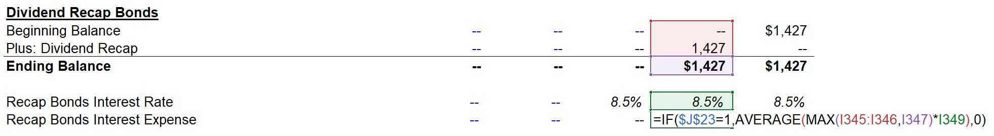
For the interest expense calculation, the minor difference mentioned above will make the calculation a bit less convenient.
First, we will start with a circuit breaker as with all interest expense calculations. Then, we will take the “AVERAGE” between the:
- “MAX” between the “Beginning Balance” of the Recap Bonds and “Plus: Dividend Recap”
- The “Ending Balance” of the Recap Bonds
And then we will multiply by the interest rate of 8.5% as shown below:
In the last step, we will calculate the “Recap Bonds Financing Fees Amortization”, which is just calculated as “MAX” between the “Beginning Balance” and “Plus: Dividend Recap” multiplied by the 2% Financing Fee assumption and then divided by the Financing Fee Amortization Period of 8 years.
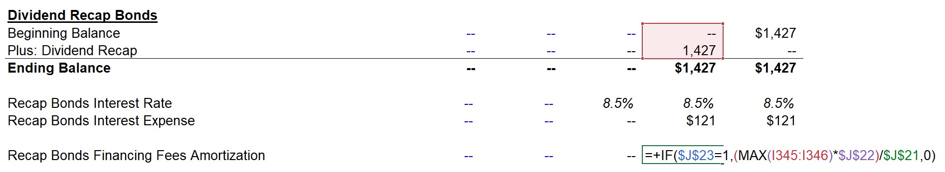
The reason we keep using the “MAX” function for the recap debt is that we do not know when the recap is done, therefore we have no other option but to do this.
As we mentioned earlier that we would have to return to this, the “Recap Bonds Financing Fees Amortization” will be added to the “Amortization of Financing Fees & OID” in the financial build.
Finalize Financial Forecast
Now that the debt schedule has been completed, we can return the financial forecast to account for portions skipped over (e.g. interest, mandatory amortizations, cash sweep, and the dividend recap/draw).
The interest, mandatory amortization, and cash sweep should be very straightforward as you are just linking or summing up the relevant cells directly from the debt schedule.
For the “Plus: Recap Senior Notes Draw”, we will link to the recap debt schedule and pull the new debt amount raised for the dividend. Then, right below it will be reflected as an outflow of the same amount as a one-time special dividend to the shareholders in the “Less: Recap Dividend Issuance”.
Thus, the net impact on cash should be zero since the two will offset each other in effect.
Note: This is unrealistic but usually how it is done in model tests. In real life, you would have lender agreements that restrict a dividend without refinancing (or some other type of compensation/adjustment to the debt terms, etc.). But in our hypothetical scenario, there is only one lender, and the sponsors have received the approval of this dividend.
Step 9. Capitalization Table
Before we can begin to calculate the returns on WSPCP’s investment, we must first determine the initial ownership structure and how the percentages change on a diluted basis.
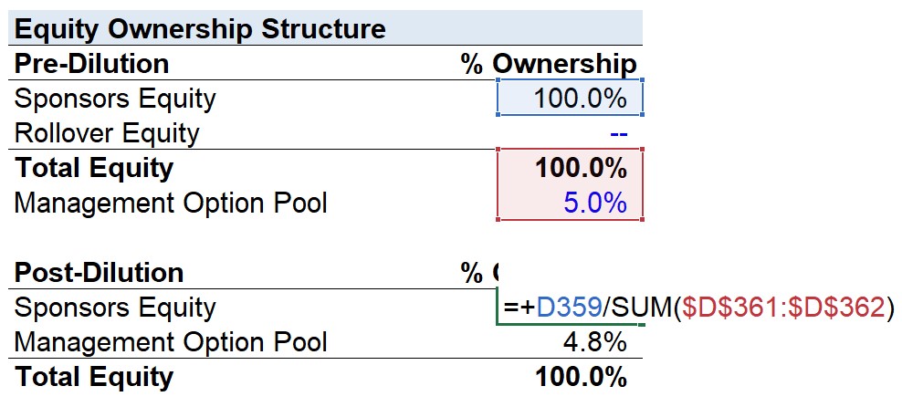
- Pre-Dilution Equity: Because there was no rollover equity and the existing management was replaced, the sponsor ownership is 100%, which includes the equity contributions from the Lead Sponsor and WSPCP.
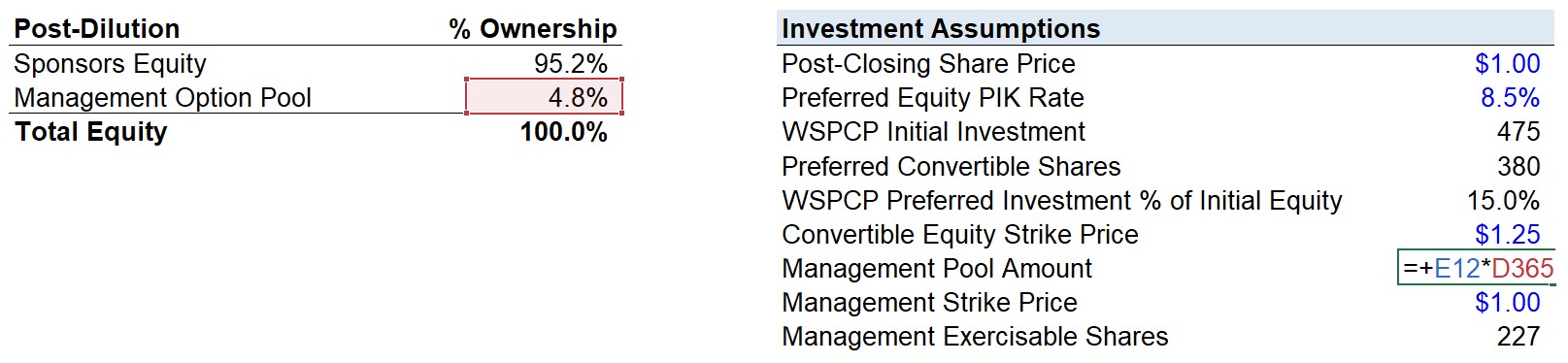
- Post-Dilution Equity: Since there’s a 5% option pool, we’ll divide the pre-dilution ownership by 105% to arrive at a post-dilution ownership of 95.2% for the sponsors.
Management Option Pools
There are two approaches to calculating the value to management from options.
Approach #1: Percentage of Full Exit Value
Most LBO Model Tests will assume the option pool is fully executed, so to determine how much value goes to management you would just multiply the entire exit equity value by the post-dilution management ownership for each year in the calculation of the return.
Let’s say there is only one sponsor, and the post-dilution sponsor ownership percentage is 90.9% (i.e. the management rollover and options pool equates to 10%). The exit equity value attributable to the sponsor would be calculated by multiplying the total exit equity value by 90.9%, and the amount that goes toward the management team is calculated by multiplying the total exit equity value by 9.1%.
Approach #2: Percentage of Exit Value in Excess of Original Investment
Alternatively, the management pool may just be based on the excess equity value creation over the initial equity investment (from the Sources & Uses schedule), thus you would multiply the excess by the agreed-upon percentage (e.g. 10%) each exit year. So you first deduct the initial sponsor investment amount from the exit equity value (i.e. the excess) and then multiply this amount by 10%. The fixed 10% payment for the excess is used and not adjusted for dilution (although the sponsor ownership dilution has changed).
Other Approaches
While the two approaches described above are the most common, there are other variations. For example, management equity can be structured such that management is to receive 10% of equity exceeding 2.0x sponsor equity. Then, the amount to management would be calculated as 10% of the exit equity value less the 2.0x initial sponsor investment.
Option pools for management teams are highly negotiated forms of compensation and there are many variations out there, so you need to identify and be sure you understand how it was structured to correctly model the returns. As a broad generalization, option pools based on the excess of the initial investment (e.g. 1.0x, 2.0x) tend to be for LBOs where existing management stayed on and rolled over some equity, while structures based on actual ownership tend to be more common when a new team is brought on since they quite literally own zero equity on paper.
For our JoeCo example, a strike price was actually provided so we cannot just assume execution of the options without actual value creation (i.e. > $1.00 implied share price). And since there was no mention of the proceeds being based on the excess equity value over the sponsors’ initial investment, we can assume this will be based on the full exit equity value. This is why we calculated the post-dilution percentage of 4.8% as this is a new reservation of ownership, and thus the +5% to the 100%. The intuition is that as long as there is value creation, the management will own 4.8% of the entire exit equity value of JoeCo.
Investment Assumptions
How many shares does the Lead Sponsor own then? We divide the initial investment by the “Post-Closing Share Price” of $1.00 (per the Prompt).
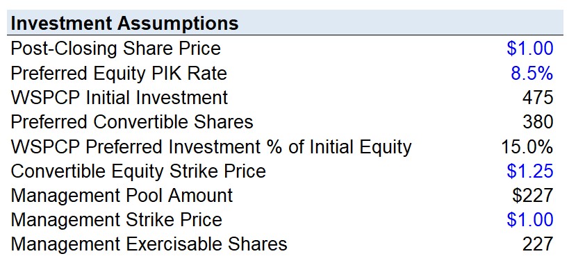
Post-Closing Share Price: The $1.00 “Newco” share price is arbitrary and at the discretion of the new ownership (e.g. Lead Sponsor, WSPCP). What matters is the equity value of JoeCo and the ownership structure percentages, which will remain completely unchanged.
Armed with the closing share price, we can outline the initial number of common shares outstanding.
There was no rollover equity and 100% of WSPCP’s co-investment was in the form of preferred stock, NOT common stock so the Lead Sponsor owns 100% of the common shares outstanding – at least initially.
Getting back to the investment assumptions…
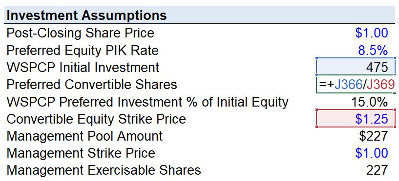
Preferred Convertible Shares: Represents the number of common shares WSPCP would own if it chooses to convert to common rather than receiving the accrued value of the preferred stock.
Just how many common shares can WSPCP own? The amount will be calculated by dividing the “WSPCP Initial Investment” by the “Convertible Equity Strike Price” of $1.25, which yields 380mm.
- WSPCP Preferred Investment % of Initial Equity: Calculated by dividing the WSPCP initial equity investment by the total equity amount. The percentage of total equity (common + preferred) at purchase owned by WSPCP is 15%, while the other 85% was contributed by the Lead Sponsor. This will come into play when calculating the amount of the recap dividend that will be distributed to WSPCP, as this is the assumption provided by the prompt (i.e. WSPCP will receive 15% of the recap dividend).
- Management Assumptions: First, the “Management Pool Amount” will be calculated by multiplying the management’s 4.8% diluted ownership by the entry valuation.
Like we did for WSPCP, we will determine the number of exercisable shares owned by management by dividing the “Management Pool Amount” by the “Management Strike Price” of $1.00.
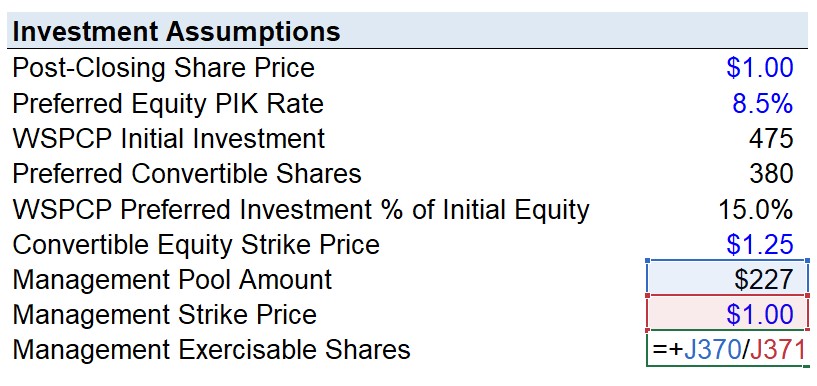
Assuming management’s options are “in the money” as of the exit date, they would own 227mm shares.
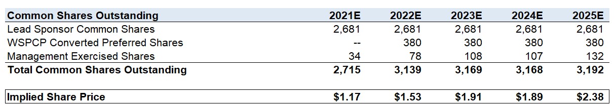
Capitalization Table
We can now bring this all together to create a mini-capitalization table (and eventually calculate the “Implied Share Price”).
“Lead Sponsor Common Shares” is simply what we calculated at the beginning of this step and will just be straight-lined since they are ordinary basic shares.
Moving on, we will calculate the next two lines, the “WSPCP Converted Preferred Shares” and the “Management Exercised Shares”, in which we already have all the necessary inputs for the calculations used in the table.
You should recognize where the 380mm and 227mm are coming from, as they represent the number of common shares created if WSPCP converts its preferred equity and if management’s options are ITM.
The formula for WSPCP’s converted share is: ” If the convertible preferred equity value is greater than the accrued preferred equity value, then the preferred convertible share count is 380mm.
Based on our prior explanations of the convertible feature of WSPCP’s preferred equity, you should be able to infer what the “IF” function is referring to. The formula says that if the value of the convertible shares is greater than that of the accrued value, then the option to convert will be selected and 380mm shares will be issued to WSPCP. The two values mentioned that will be compared have not yet been calculated and will be determined in the final step, but we did want to define them.
This formula is essentially the same as above. It states that if the “Implied Share Price” is greater than the “Management Strike Price” of $1.00, then the 277mm in “Management Exercisable Shares” will be ITM and thus issued.
But do keep in mind, the table above calculates the “Total Common Shares Outstanding” as of exit dates. These converted and exercised shares do not carry over into the next year – we wanted to make this point clear in case there might be some confusion.
Step 10. Returns Calculation
Exit Valuation
In the final step, we’ll calculate and assess the returns on WSPCP’s preferred equity investment into JoeCo.
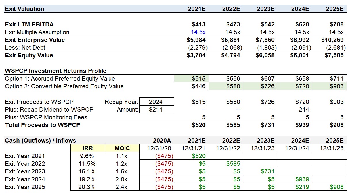
To determine the exit equity value, we will first apply an exit EBITDA multiple assumption.
For each year, we will link each Exit LTM EBITDA from the pro forma financial forecast and use an “Exit Multiple Assumption” of 14.5x, the conservative assumption provided by the prompt.
With the equity value established, we now need to establish whether, based on our model, WSPC will prefer to convert their preferred equity to common or whether they would prefer to simply keep their investment in the form of preferred stock.
Since the decision to convert is entirely the choice of WSPC, they will simply pick the choice that generates the higher return for them:
To determine this, we will first calculate the value of the preferred equity under the PIK interest of 8.5% and then the returns if WSPC does indeed convert:
- Returns if WSPC Keeps its Preferred Stock: The initial equity investment of $475mm by WSPCP will accrue each year at the 8.5% PIK rate and reaches $714mm by 2025.
- Returns if WSPC Converts: The convertible value of WSPCP’s preferred equity investment requires us to multiply the “Preferred Convertible Shares” of 380mm by the “Implied Share Price” of the relevant year.
Because of WSPC’s two options, calculating the “Implied Share Price” can be a bit trickier:
- If WSPC keeps its preferred stock, the Implied Share Price = (Equity Value – WSPC Preferred Stock)/Common Shares
- If WSPC converts, the Implied Share Price = Equity Value/(Common Shares including the dilution from the newly converted shares to WSPC)
Since the resulting share price determines the value of the if-converted preferred equity, we also have a circularity that requires we insert a breaker.
- Convertible Value > Accrued Value: The formula states, if the “Convertible Preferred Equity Value” is greater than the “Accrued Preferred Equity Value”, then the “Implied Share Price” is calculated by dividing the “Exit Equity Value” by the “Total Common Shares Outstanding”.
- Accrued Value > Convertible Value: On the other hand, if the “Accrued Preferred Equity Value” exceeds the “Convertible Preferred Equity Value”, we deduct the “Accrued Preferred Equity Value” from the “Exit Equity Value” and then divide this amount by the “Total Common Shares Outstanding”.
Based on our model assumptions, conversion is the optimal choice for WSPC post-2021, which we determined via the “MAX” function between the two options to output the one of greater size between the two.
For the dividend recap, we will first multiply the “Less: Recap Dividend Issuance” from the financial forecast by the pre-dilution ownership percentage of 15% we listed in the “Investment Assumptions” section. The reason we use the pre-dilution percentage is that this was before the exit and the management pool had no dilutive impact on the equity ownership structure. Also, the prompt stated to do this specifically.
So if a dividend recap is completed in 2024, the dividend amount to WSPCP is $214mm, but we need to ensure 2025 reflects this dividend received too.
- Recap Dividend to WSPCP: For the “Plus: Recap Dividend to WSPCP”, the formula used is shown below for 2025. It is essentially saying that “IF” the current year is equal to the recap year, then the dividend amount will be added to the “Total Proceeds to WSPCP” line item.
- WSPCP Monitoring Fee: For “WSPCP Monitoring Fee”, it is faster to just do it manually and confirm you linked it properly. It is $5mm each year received for consulting services to JoeCo. The monitoring fee is paid out annually and should thus be linked to each individual year prior to the exit. But be sure not to double-count it, and sanity check you did properly by confirming for Exit Year 5, $25mm in total was received in fees.
Sensitivity Analysis (IRR and MOIC)
We can now calculate the IRR using the XIRR function and MOIC by dividing the proceeds by the initial investment.
If we assume a year 5 exit under our base case assumptions, we arrive at the following return profile.
- IRR = 20.3%
- MOIC = 2.4x
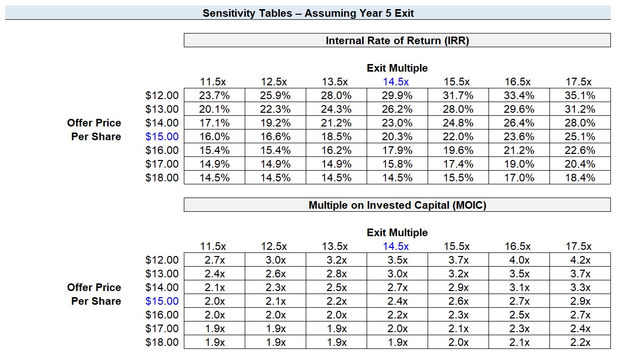
In the final step before we answer the questions, we will perform sensitivity analysis on the IRR and MOIC. The process is the same as usual, the only difference is the variable on the left will be the offer value per share rather than the entry multiple.
LBO Modeling Tutorial Conclusion
In closing, here are some sample questions that could’ve potentially appeared in the prompt:
- Q. Do you think the benefits of investing in the preferred equity of JoeCo were worth it, as opposed to just investing in the vanilla common equity?
- Q. Why do you think WSPCP decided to invest in the preferred equity of JoeCo? Do you think there were sufficient risks for this required downside protection?
- Q. What is the relationship between the timing of the dividend recap and the add-on acquisition, and if the decision was mutually exclusive – which one would you recommend to the firm?
- Q. WSPCP contributed only $475mm into this take-private of JoeCo, if the decision was up to you – would you have invested more capital? (Hint: Recap Dividend)
- Q. If you wanted to understand whether this was actually a “good” investment for WSPCP, what three questions would you ask the investment committee of WSPCP?
We will intentionally not provide direct answers to these questions, albeit we have already discussed most of them. But do keep these questions in the back of your mind as you complete the model and as you adjust the assumptions to see how the returns change.
As you can deduct from all the commentary throughout this article, while there are many wrong ways to build a model like this, there isn’t only one correct answer, and if you were to look at the models submitted by ten different candidates, they would all vary, and the IRRs/MOICs would marginally deviate from one another.
For instance, the date that the dividend recap is accounted for in the returns schedule is technically incorrect (i.e., year-end), as the recap was assumed to be received at the beginning of the period. However, the relative impact on fund returns is insignificant and not enough to actually influence the investment decision.
While these sorts of simplifications would certainly not pass on the job, for purposes of LBO modeling tests in the interview setting, some minor “shortcuts” are acceptable for the sake of conserving time. Note, you also need adequate time to prepare for the discussion right afterward, especially since the model will not be in front of you when discussing your thoughts on the investment.
Above all else, prioritize the full completion of the model and focus on the key variables that have real implications on returns.
Those factors will ultimately determine the final recommendation and serve as the main discussion points upon submitting the model, rather than minor modeling quirks that cause <1% differences in the IRRs.
The model does not have to be perfect, nor is it expected to be, but your attention to detail, ability to see the big picture and decision-making under pressure are what is being assessed in the quality of your work.


Hi, Thank you for the thoroughness. I have one question regarding the intangible asset write up – the pre-LBO intangible asset on the book is 0. So why is the intangible asset write up = allocable purchase price premium x 10% instead of pre-LBO book value of intangible assets x… Read more »
Hi WSP team, The prompt states that the maximum leverage multiple is 6.0x however in the solutions tab when you complete the acquisition of TeaCo in 2021 the new debt from the revolver would put you over the 6.0x limit when combined with the unitranche. Am I misunderstanding how the… Read more »
Hi there, I don’t quite understand how we can earn on a positive IRR for a transaction that goes from $12-15 share price to ~$1 implied share price at the end makes sense.
Hi, thank you for coming up with the amazing material! Are we missing 1 row of PIK interest deduction from the income statement and the corresponding add-back in the cash flow statement, or should this be treated differently from what we see in the standard model? Thank you!
Shouldn’t the post dilution option pool equal 5%? Using shares and a 10% option pool- Let’s use 100 in your example. Sponsor gets 100 shares at $1 / share. A 10% pool means management gets 10% of the company, excluding the impact of strike, but including the option dilution. Therefore,… Read more »
Hey there, thank you for this extremely helpful tutorial! I have one general question. How common are the following case scenarios in final-round modelling tests for upper mid-market funds (ideally, if someone has knowledge on European interviews): 1) Dividend recap 2) Management option pool 3) Management earn-outs 4) Add-on acquisition… Read more »
Thanks for the great write up, this is one of the best LBO case study walk-throughs I’ve come across so far. Is the Recap Bonds Interest Rate (Line 350) formula correct? Looks like it’s only taking the average of one input, if we’re trying to obtain the average interest expense… Read more »
Hi, Thanks for the model and article, they are great. Just want to confirm that for line 377 – Management Exercised Shares, it is calculated using TSM as opposed to a straight conversion? The former was related in the completed file while the latter was reflected in the screenshots under… Read more »
Hey, Why is the management pool amount calculated with the equity value pre LBO? (E12). The equity value pre LBO is based on a different capital structure. Shouldn’t the management pool be the product of management’s diluted share (4.8%) and equity value at entry but PF for the LBO capital… Read more »
Hey, thanks for the case study!
You have deducted the $119m of transaction expenses from the equity, why are the transaction expenses not tax deductible? Shouldn’t you subtract the after tax amount?
Hi, the capitalized financing fee is under liability for PF B/S – shouldn’t the capitalized financing fees be recognized as an intangible asset?
Hi, Firstly, thanks for this. The materials here are very comprehensive and useful in understanding all the LBO quirks! I just had one question on the dividend recap returns analysis. I see for the year 5 exit analysis, the dividend recap is included in the year 5 (even though the… Read more »
Hi, In the dividend recap section of the debt schedule it is mentioned that the ” “Maximum Recap Debt Capacity” for the current year will be calculated by multiplying the EBITDA of the previous year by the “Maximum Leverage Multiple” of 6.0x”, however when I look at the completed version I see that… Read more »
Thanks!
Hello, another quick question regarding this model. In your calculation of “Option 2: Convertible Preferred Equity Value”, it doesn’t seem like you checked whether the implied share price > strike price of the preferred equity value. I think to be completely accurate, you would need to check if the share… Read more »
Hi – I am curious why Intangible asset and PP&E Write up Amortization values show up as operating expenses on the P&L? Shouldn’t they be below EBIT?
Thanks,
John
HI WSP team, thanks for the informative model. I thought in share deals you are not allowed to write up assets or create DTA? In this example, we are acquiring shares rather than assets so why are we able to write up assets and intangibles?
Hello, I understand in this model we are calculating return from the perspective of WSPCP. However, if we were calculating return from the perspective of the lead sponsors, is the equity available to the lead sponsor = exit equity value – mgmt pool equity if exercised – convertible preferred share… Read more »
Hi WSP team, not sure how you solve this; but when I calculate to the last step of management pool shares, I found that the exercised shares of management rely on implied share price while implied share price is calculated based on total shares which include the exercised shares of… Read more »
Hi Tyler — our modeling test prompt states to assume so in the add-on section, which was only done in an effort to simplify the already long-winded model.
Thanks!
Hi, Thanks for this helpful tutorial I just wanted to check the rationale for not including D%A for add on acquisition in balance sheet and Cash flow statement; also not included in change in NWC Is that to simplify the model assuming the impact of those line items for add-ons… Read more »