Standard LBO Modeling Test

[toc]

Standard LBO Modeling Test: 90-Minute Practice Tutorial

The following standard LBO modeling test usually comes after the more basic “paper LBO” or technical interview questions you might encounter in earlier rounds.

If you’re completely new to this, you should start by reviewing those before moving on to a full model practice test such as our short-form LBO modeling test that precedes this intermediate-level test.

The chart below summarizes when you should expect to see PE technical interview questions and LBO tests throughout the recruiting process:

Type	Description
Technical Interview Questions	For investment banking analysts, you’ll likely not see a lot of these as it’s usually assumed you have this down. You’re more likely to see this in the first round if you come from a non-traditional background. See: Top 25 Private Equity Interview Questions
Paper LBO	Usually given at early rounds, you’ll be handed only pen and paper and 5-10 minutes to arrive at an implied IRR and other key metrics based on the information provided in the prompt. See: Paper LBO
LBO Modeling Test	The LBO Modeling Test is a near certainty at later rounds. The level of difficulty will, however, vary and can be broken up into 3 broad buckets: Basic LBO Modeling Test – A relatively easy practice test that usually takes around 45 minutes (and an hour at most). If you’re finding the standard test in this article to be difficult, you should go back and start with this one. Standard LBO Modeling Test (*This Tutorial*)– This is the level of difficulty that we’re going to cover here in this post. You’re usually given about 1-hour minimum (and up to 2 hours at the most). At traditional lower-middle market funds, you may only be given this Standard Model Test, while mega-funds and upper-middle market funds are known for giving more advanced modeling tests – albeit, this can differ by each recruiting cycle. Advanced LBO Modeling Test – You’re most likely to see this from the mega-funds or upper-middle market funds, especially for those categorized as “specialists” (e.g. special situations). Can be given as much as 4 hours.

How Important is the LBO Modeling Test?

Doing a good job on this test is not – on its own – enough to receive an offer. However, a lackluster submission may be the reason you don’t receive an offer.

To get the offer, you’ll also need to ace the behavioral portion of the interview, deal (or investment) discussion, and case study.

How Are Modeling Tests “Graded”?

The grading system is pretty straightforward and could be best described as “check the box”. The person responsible for reviewing your model, most often one of the younger associates, will not be questioning your assumptions or assessing your ability to interpret the model.

But rather, the associate is confirming the instructions were correctly followed. If the model was built properly, the process of reviewing your work should take no more than fifteen minutes at most. As such, a huge part of doing well under stress is attention to detail.

Basic vs. Standard Level LBO Modeling Test

So, how does the structure of this model differ from the more “Basic” LBO Modeling Test?

• More Time Consuming (1 to 2 Hours): Because the instructions are more extensive with more moving pieces, you will be given more time to complete the model – the caveat being, mistakes in your model are penalized more since you were given more time to go back and check your work.
• Full 3-Statement Build: To confirm you understand the financial statements linkages, you will be asked to build out the income statement, balance sheet, and cash flow statement – this can actually be beneficial because it provides you with more opportunities to check your model and catch mistakes (i.e. if the B/S doesn’t balance, you made an error somewhere).
• Additional Features: In the Basic LBO Modeling Test, we introduced the core mechanisms of an LBO model such as the Sources & Uses table, the free cash flow build, a simplistic debt schedule (e.g. revolver mechanics, floating vs. fixed pricing, mandatory amortization), and returns calculation. In this practice test below, we’re going to add a few features you should be ready for, as they are commonly tested, including:
  • Rollover Equity
  • Purchase Price Allocation (Closing B/S, Goodwill Creation, DTLs)
  • “Cash Sweep” Optionality
  • Modeling PIK Interest
  • Sponsor Monitoring Fees
  • Returns Sensitivity Analysis

LBO Modeling Test Prompt Example

Let’s now get straight into the model tutorial. Keep in mind that, unlike the previous article, we will presume you have a decent understanding of Financial Modeling Best Practices and the mechanics of an LBO model – i.e. we will not be explaining the circularity toggle, revolver functionality, etc.

LBO Model Instructions

A private equity firm is evaluating a potential leveraged buyout of JoeCo, a privately held coffee company. In the last twelve months, JoeCo generated $715mm in revenue and $50mm in EBITDA.

Assume the PE firm acquired 80% of JoeCo’s equity at an entry multiple of 12.5x LTM EBITDA with the remaining 20% being rolled over by the existing management team.

Based on the assumptions provided below, calculate the IRR and MOIC from the investment with an operating 3-statement model and provide answers for the following questions:

Questions

1. What is the implied IRR and MOIC if the PE firm exits JoeCo at the same multiple as entry in a five-year horizon?
2. At what multiple would the PE firm need to exit JoeCo at to achieve a 3.0x MOIC after a five-year holding period?
3. If the firm’s minimum IRR threshold is 15%, what is the lowest multiple the PE firm could sell JoeCo at while still meeting the return hurdle?

Operational Assumptions

• LTM Revenue was $715mm and is expected to grow 8% in 2021 – then in the years onward, the growth rate will increase incrementally by 0.5% each year
• LTM Gross margin was 31.5% and this figure is expected to increase by 0.2% each year
• SG&A, R&D, and D&A as a percentage of revenue will remain constant throughout the entire holding period (i.e. SG&A: 21%, R&D: 3.5%, and D&A: 1.4%)
• Capex as a percentage of revenue will be 2.0% each year
• An annual monitoring fee of $2mm will be paid to the private equity firm
• Use a tax rate of 35%

Transaction Assumptions

• Entry multiple to purchase JoeCo was 12.5x LTM EBITDA
• Date of transaction closing was 12/31/2020
• Transaction fees paid to the investment banks, consultants, and accountants were $10mm
• Cash to B/S will be $5mm
• Existing management team has agreed to rollover 20.0% equity
• Financing fees will be 2.5% for all debt tranches (excluding the revolver) and will be amortized over a 7 year period
• Intangible assets will be written up as 10.0% of the purchase premium with a useful life assumption of 15 years
• PP&E was written up 20.0% from its LTM balance with a useful life assumption of 10 years

Financing Assumptions

• Revolving credit line (“Revolver”) was left undrawn at purchase, priced at LIBOR + 400, the max capacity is 75% of LTM Inventory and AR, and the unused commitment fee is 0.25%
• Term Loan B (“TLB”) was raised at 3.5x EBITDA, priced at LIBOR + 400 with a 2% Floor, 5% mandatory amortization, and 100% cash sweep
• Senior Notes were raised at 1.5x EBITDA and has an interest rate of 7.0%
• The final debt tranche used were Subordinated Notes (“Sub Notes”), which were raised at 1.0x EBITDA – carries a 12.5% interest rate, of which 8.5% is cash interest and 4% is paid-in-kind (“PIK”)
• There is no prepayment optionality for neither the Senior Notes nor the Sub Notes
• Assume all debt instruments have a 7 year term

LBO Modeling Test – Excel Template

AMEX

First Name *

Email *

Submit

By submitting this form, you consent to receive email from Wall Street Prep and agree to our terms of use and privacy policy.

Email provided

Your Download is Ready

Submitting...

As you can see in the “Financials” tab, the LTM income statement and balance sheet of JoeCo were provided. This is the format the financials will generally be provided in. For short tests, the prompt is usually written out near the financials in 5-10 bullet points. But for longer model tests (such as this one), the prompt is typically provided separately in either a Word doc or PDF.

Step 1. Model Assumptions

Entry Valuation

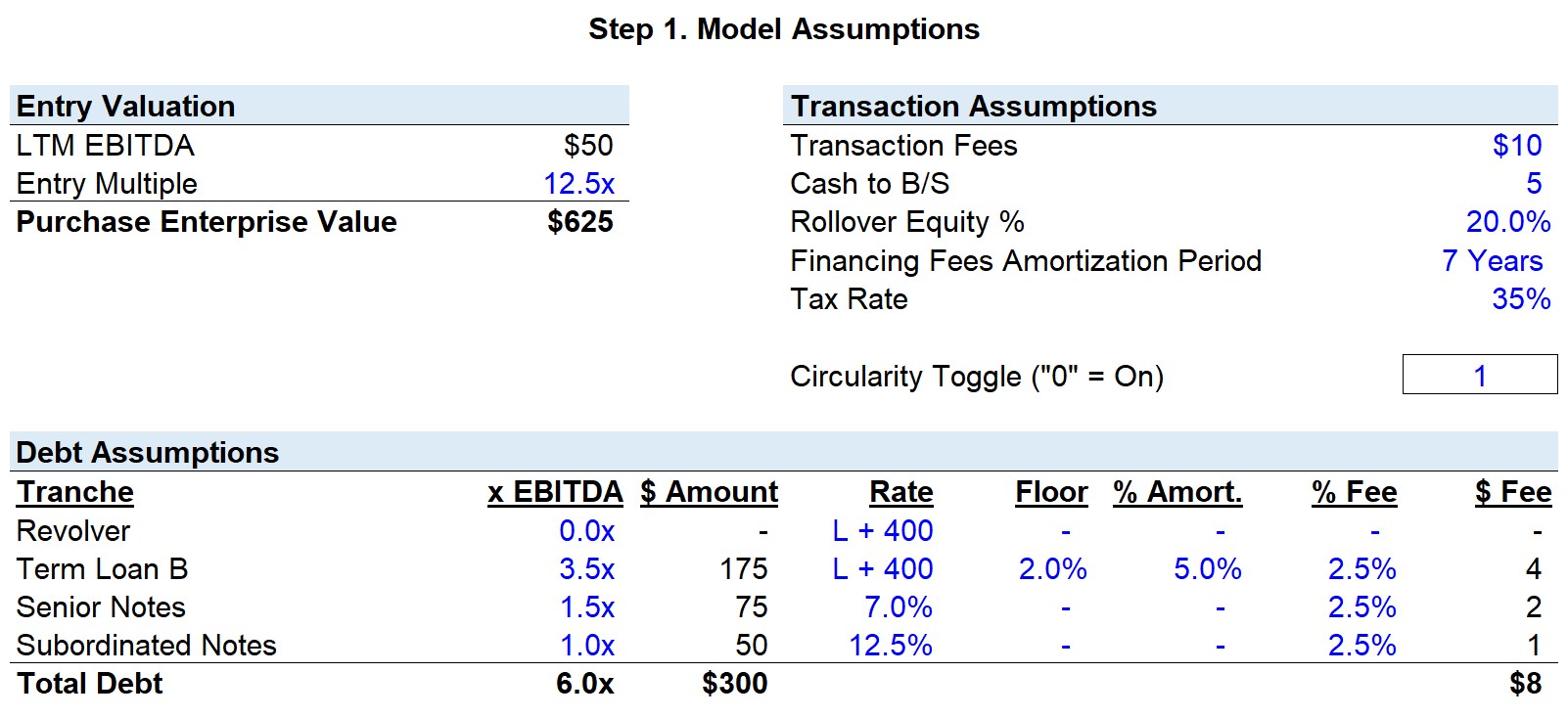
Per usual, the first step to building an LBO model is to determine the initial valuation of the company at purchase. Since this deal was completed on a “Cash-Free, Debt-Free” Basis, the purchase price will be equal to the purchase Enterprise Value (“TEV”).

JoeCo’s LTM EBITDA is $50mm and the entry multiple paid was 12.5x – thus, the purchase enterprise value is $625mm.

Transaction Assumptions

Moving onto the transaction assumptions, the transaction fees were $10mm, Cash to B/S is $5mm, financing fees amortization period is 7 years, and the tax rate to be used is 35%.

The one new line item included is “Rollover Equity %”, which amounts to 20% as given by the prompt.

Rollover equity means the management team of JoeCo has decided to carry over a portion of their existing shares into the recapitalized company to participate in the potential upside of this LBO.

As a side note, in this particular scenario, the 20% does NOT mean that management is rolling over 20% of their pre-LBO equity, but rather their rollover will represent 20% of the post-LBO equity (i.e., plug the remaining equity needed).

Since the sponsor’s investment is 80% of the required equity contribution, then the management rollover comprises the rest, the leftover 20%.

In the prompt, we are specifically told the sponsor holds an 80% implied ownership stake, which is a sign that the rollover equity can be calculated using this simplified approach. When it comes to basic and standard LBO modeling tests, this method is very common to see, the other being a hardcoded amount.

Debt Financing Assumptions

To finish the model assumptions section, the remaining portion is the debt assumptions table that lays out the terms of the various debt instruments used.

• The leverage multiples by debt tranche were 3.5x for Term Loan B (“TLB”), 1.5x for the Senior Notes, and 1.0x for the Subordinated Notes (“Sub Notes”)
• This amounts to total leverage of 6.0x, meaning $300mm of debt was raised to fund the purchase of JoeCo. To break this amount out by tranche:
  • $175mm raised via TLB
  • $75mm raised via  Senior Notes
  • $50mm raised via Sub Notes
• Revolver and Term Loan B are priced at a floating rate of “LIBOR + 400” with the TLB having a floor of 2%.
• The TLB is the only debt tranche with required amortization payments of 5% each year with a full 100% cash sweep.
• Senior Notes and Sub Notes are both priced at fixed rates – 7.0% and 12.5% respectively
  • One notable difference is that only 8.5% of the sub notes are paid-in-cash, with the remaining 4% paid-in-kind (“PIK”).

As we can see on the right side of the debt assumptions table, the financing fee % for all of the tranches of debt (excluding the revolver) is 2.5% – thus, the total financing fees incurred comes out to be $8mm, which will be capitalized and amortized over the 7-year term.

Step 1: Formulas Used

• Purchase Enterprise Value = LTM EBITDA × Entry Multiple
• Debt Raised (“$ Amount”) = Debt EBITDA Turns × LTM EBITDA
• Financing Fees (“$ Fee”) = Debt Raised × Financing Fee %

Step 2. Sources & Uses Table

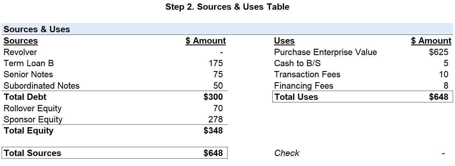
Onto the next step, we will now complete the Sources & Uses table – which outlines how much the acquisition of JoeCo will cost and how much debt and equity will be required by the private equity firm to fund the transaction.

Uses Side

Starting on the “Uses” side, we have already calculated the purchase price as $625mm and can link to the relevant “Purchase Enterprise Value” cell.

Next, the Cash to B/S is $5mm, this means JoeCo’s cash balance cannot dip below this pre-determined level post-closing and thereby increases the amount in funding required.

To finish the Uses side of the table, the transaction fees were $10mm while the financing fees were $8mm as previously calculated.

So to acquire JoeCo, the private equity firm requires $648mm in total funding.

Sources Side

The appearance of the “Sources” side of the table and the calculations will be slightly different because of the additional source of equity funding, the management rollover.

Starting with the debt tranches, we can just link the debt amounts from the debt assumptions table where we have already calculated the amounts raised based on the turns of EBITDA. In total, $300mm in debt was raised to fund this purchase.

Now we move onto the equity portion of the funding, which will amount to the remaining amount of funding required post-debt financing.

Given the existing management team has rolled over 20% equity, we must calculate the amount of the rollover in dollar terms.

But first, we must calculate the total equity contribution required from the rollover and sponsor. To do so, we take the $648mm in “Total Uses” and deduct the $300mm in “Total Debt”. This is the residual amount of equity necessary, but the key distinction is that the private equity firm did not purchase 100% of JoeCo’s equity.

The subsequent step is to multiply the 20% rollover equity assumption by the $348mm in required equity to get $70mm as the amount rolled over by the management team into the new, post-LBO entity.

Finally, to determine the initial equity investment by the private equity firm, we calculate the “plug” by deducting the $70mm in management rollover from the $348mm in required equity. So, the rollover equity is 20% of the required equity, $70mm (20% x $348mm), while the sponsor equity is 80% of the required equity, $278mm (80% x $348mm).

Once that is done, we see the sponsor contribution was $278mm and both sides of the table are now in balance.

Step 2: Formulas Used

• Total Uses = Purchase Enterprise Value + Cash to B/S + Transaction Fees + Financing Fees
• Total Debt Raised = Revolver + Term Loan B + Senior Notes + Subordinated Notes
• Total Equity = Total Uses – Total Debt Raised
• Rollover Equity = Total Equity x Rollover Equity %
• Sponsor Equity = Total Equity – Rollover Equity
• Total Sources = Total Debt + Total Equity

Step 3. Purchase Price Allocation (“PPA”)

Now that the transaction structure has been set up, the next step is to create the closing balance sheet, which refers to the pro forma balance sheet after the deal adjustments have been accounted for.

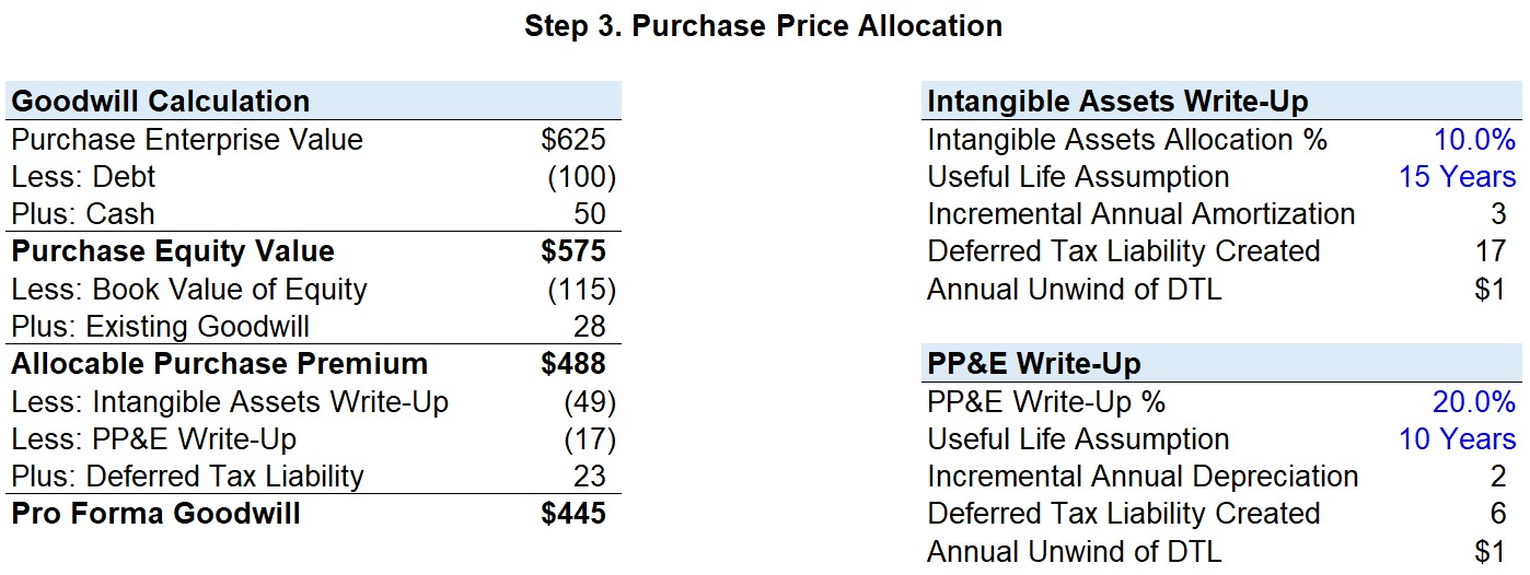
Before we can put the closing B/S together, we must first calculate the amount of goodwill created from an acquisition accounting practice referred to as purchase price allocation (“PPA”).

The purpose of PPA is to identify and assign the fair value of the acquired tangible and intangible assets and liabilities as of the date of transaction closing.

The fundamental equation of PPA sets the assets acquired and liabilities assumed equal to the value of the consideration paid before making the necessary adjustments. Once the adjustments have been made, the remaining difference between the purchase price and the fair value of the acquired assets and assumed liabilities will be recognized as Goodwill on the balance sheet.

Purchase Premium

All acquirers, whether strategics or financial buyers are required to perform purchase price allocation to disclose the fair values of the purchased assets. For nearly all cases, the purchase price will exceed the fair value of the acquired assets and liabilities (i.e. a purchase premium was paid) – thus, the resulting excess leads to the creation of goodwill.

The first step in purchase price allocation is to determine the purchase equity value. We calculated the purchase enterprise price earlier, therefore we need to deduct the net debt. Taking a look at JoeCo’s LTM financials, we see that JoeCo has $100mm in existing debt and $50mm in cash – thus, the net debt is $50mm and the purchase price to acquire 80% of JoeCo’s equity was $575mm.

In its simplest form, the pro forma goodwill is calculated as the purchase equity value minus the book value of equity plus the existing goodwill. The reason we wipe out the existing equity book value is that it no longer exists (i.e. will be replaced by the new equity investment) and then we add existing goodwill because we would be double-counting it if we did not.

The rationale behind why we wipe out the existing equity shareholder value and goodwill will make more sense later when we walk through the closing B/S.

So if we take the $575mm in purchase equity value, subtract the book value of equity of $115mm, and add the $28mm in existing goodwill – we arrive at a purchase premium of $488mm. If there are no other fair value adjustments, this would be the total amount of goodwill created that would then flow into the closing B/S.

Put another way, this is the total amount of goodwill required to properly function as the “plug” for both sides of the closing B/S to balance.

Pro Forma Goodwill

Notice in our model, the line item that captures the excess of the fair value of the assets over the book value is named “Allocable Purchase Premium”.

The reason being, the purchase premium (and the amount of goodwill created) can be affected by the write-ups / write-downs during the acquisition accounting process.

In this example, the prompt mentioned two adjustments that will impact the goodwill created in this transaction: 1) Intangible Assets Write-up and 2) PP&E Write-up

So, what are the implications of intangible asset and PP&E write-ups on the creation of goodwill?

Since goodwill is meant to plug the difference between the purchase price and fair value of the assets in the closing B/S – a higher write-up implies the assets being purchased are actually worth more. In other words, the valuation appraisers determined that the intangible assets and PP&E of JoeCo are worth more and therefore need to be appropriately adjusted on the closing B/S to better reflect their fair value.

As a result – the more JoeCo’s intangible assets and PP&E are written up, the less goodwill will have to be created on the date of the transaction.

Intangible Assets Write-Up

Oftentimes, acquired intangible assets such as patents, intellectual property (IP), trademarks, customer/supplier relationships (i.e. contracts) can be revalued and written up in value.

Here, the write-up of the intangible assets has been provided as 10.0% of the allocable purchase premium. If we multiply the write-up percentage assumption of 10.0% by the purchase premium of $488mm, we get to $49mm as the intangible assets write-up.

Since write-ups reduce the amount of goodwill created, a minus sign must therefore be placed in front of the formula.

Another implication of the write-ups of intangible assets is the increased amortization. The useful life of the intangible assets was provided as 15 years, therefore we can divide the $49mm by 15 to get an incremental amortization expense of $3mm each year.

PP&E Write-Up

Next, we will calculate the write-up of JoeCo’s PP&E. The percentage assumption for PP&E is 20.0%, but this was stated in terms of a step-up of the existing PP&E balance rather than a percentage of the allocable purchase premium like the intangible assets.

Therefore, we will multiply the LTM PP&E balance of $83mm by 20.0%, which comes out to $17mm in this case.

Given the useful life assumption of 10 years, the annual incremental depreciation from the PP&E write-up is $2mm.

Deferred Tax Liability (DTL)

We have now calculated the write-up amounts and the associated depreciation/amortization expenses, but the tax implications must not be forgotten. Specific to this LBO of JoeCo, deferred tax liabilities (DTLs) are created from the PP&E and intangible assets being written up.

Deferred taxes arise when there is a temporary timing difference between GAAP book taxes and the actual cash taxes paid to the IRS, which has a direct impact on the amortization expense (and GAAP taxes).

If cash taxes in the future exceed book taxes in the future, a deferred tax liability (DTL) would be created on the balance sheet to offset this temporary tax discrepancy.

While the additional depreciation stemming from the PP&E write-up and the amortization of intangibles are deductible for book purposes, they are not deductible for tax purposes.

Eventually, GAAP taxes will increase accordingly once these temporary timing differences are eliminated.

To calculate the deferred tax liability created from the intangible assets write-up, we will multiply the $49mm write-up by the tax rate of 35% to get $17mm.

To calculate the deferred tax liability created from the PP&E write-up, we will multiply the $17mm write-up by the 35% tax rate to get $6mm.

The total deferred tax liability associated with the two write-ups comes out to $23mm. The annual “unwind” of the DTL will be calculated by dividing the DTL created by the useful life assumption.

Be aware, that the annual unwind of the DTL is calculated separately and then summed up since the two write-ups have differing useful life assumptions.

In closing, the total amount of goodwill created was $445mm. This was calculated by taking the purchase premium of $488, subtracting the $49mm in intangible assets write-up and the $17mm in PP&E write-up, and adding the $23mm in deferred tax liabilities.

Step 3: Formulas Used

• Allocable Purchase Premium = Purchase Equity Value – Book Value of Equity + Existing Goodwill
• Pro Forma Goodwill = Allocable Purchase Premium – Intangible Assets Write-Up – PP&E Write-Up + Deferred Tax Liability
• Deferred Tax Liability (DTL) = Write-Up Amount x Tax Rate %
• Intangible Asset Write-Up = Intangible Assets Allocation % x Allocable Purchase Premium
• PP&E Write-Up = PP&E Write-Up % x LTM PP&E
• Annual Incremental Depreciation = PP&E Write-Up ÷ Useful Life Assumption
• Annual Incremental Amortization = Intangible Assets Write-Up ÷ Useful Life Assumption
• Annual Unwind of DTL = Deferred Tax Liability Created ÷ Useful Life Assumption

Step 4. Closing Balance Sheet

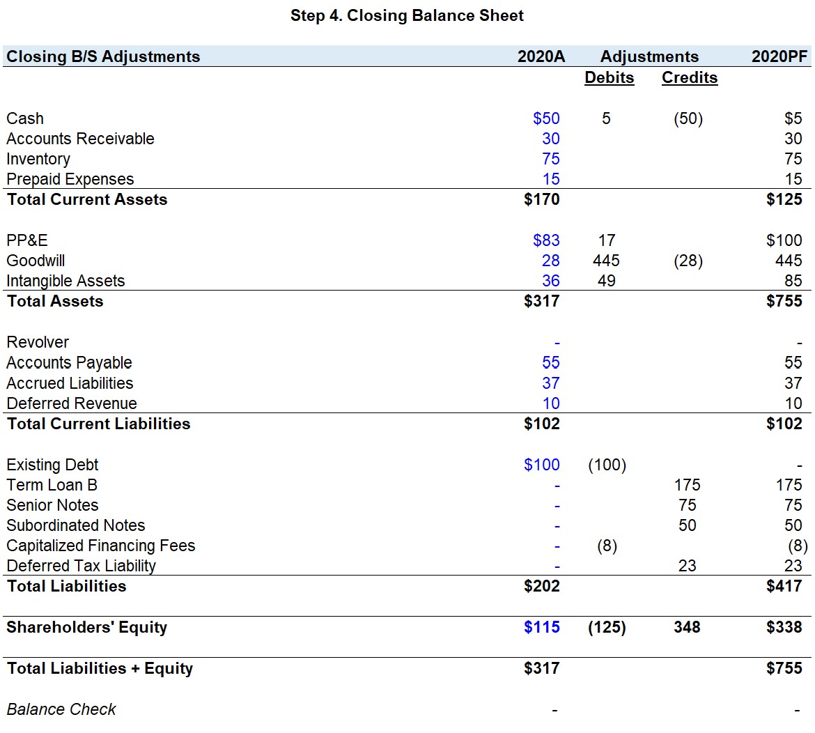
Now that we have calculated the pro-forma goodwill as $445mm and have the amount in deferred tax liabilities created, we can now put together the closing B/S.

Assets Side

The first adjustment will be wiping out the entire cash balance on the credits side (-$50mm) since this deal was done on a CFDF basis. Then, on the debits side we will link to the Cash to B/S from the Sources & Uses schedule (+$5mm). If you sum up the 2020A balance with the debit and credit entries, the 2020PF cash balance is $5mm – i.e. the seller took all the excess cash and the minimum cash balance remains.

Next, PP&E was written up by $17mm and this will be reflected on the debits side (+$17mm). The 2020PF PP&E balance has changed from $83mm initially to $100mm.

Moving onto goodwill, the existing goodwill of $28mm will be wiped out on the credits side (-$28mm). Next, the $445 we calculated in the previous step will be linked on the debits side (+$445mm).

For the final adjustment on the assets side of the balance sheet, the intangible assets write-up of $49mm will be reflected on the debits side (+$49mm). The PF balance has increased from $36mm to $85mm.

Liabilities and Equity Side

Moving onto the liabilities side, the first adjustment is the elimination of the $100mm in existing debt on the debits side (-$100m). Again, this deal was done on a CFDF basis, thus it is the seller’s responsibility to take care of this obligation using the sale proceeds.

Next, we will add the new debt funding raised to the closing balance sheet. On the credits side, we can link to the $175mm in TLB, $75mm in Senior Notes, and $50mm in Sub Notes (+175mm, +75mm, +50mm)

Then, we need to account for the capitalized financing fee of $8mm on the debits side (-$8mm).

To finish the adjustments on the liabilities side of the balance sheet, the Deferred Tax Liability of $23mm will be reflected on the credits side (+$23mm). This is a temporary timing difference that will gradually wind down to zero.

To finish the closing B/S, we will adjust the shareholders’ equity balance. On the debits side, we will wipe out the existing amount by entering a negative sign and then linking to the book value of equity cell (-$115mm) and then we deduct the $10mm in transaction fees (-$10mm). These transaction fees, unlike financing fees, are treated as one-time expenses and come out of equity. The debits side should now be negative $125mm.

Then on the credits side of equity, we will link to the equity contributions from the Sources & Uses table (+$348mm). In total, the 2020PF shareholders’ equity balance should be $338mm.

If done correctly, the PF closing B/S should balance. If not, it is likely an error related to the debits and credits signs. Make sure that on the debits side, all the asset adjustments are shown as positives and the liabilities and equity adjustments are shown as negatives (and vice versa for the L&E side).

Step 4: Formulas Used

• Column 2020PF: SUM (2020A, Debits, Credits)
• 2020PF Cash = 2020A Cash + Cash to B/S – 2020A Cash
• 2020PF PP&E = 2020A PP&E + PP&E Write-Up
• 2020PF Goodwill = Pro Forma Goodwill – 2020A Existing Goodwill
• 2020PF Intangible Assets = 2020A Intangible Assets + Intangible Assets Write-Up
• 2020PF Existing Oldco Debt = 2020A Existing Debt Balance – Existing Debt Balance
• 2020PF TLB, Senior Notes, Subordinated Notes: $ Amount Raised from Sources & Uses Table
• 2020PF Capitalized Financing Fees: – (Total Financing Fees Amount)
• 2020PF Deferred Tax Liability = 2020A DTL + New Deferred Tax Liability Created
• 2020PF Shareholders’ Equity = 2020A Equity – 2020A Equity – Transaction Fees + Rollover Equity + Sponsor Equity

Step 5. Income Statement

With the purchase accounting and closing B/S complete, we can now forecast the three financial statements beginning with the income statement.

Operating Assumptions

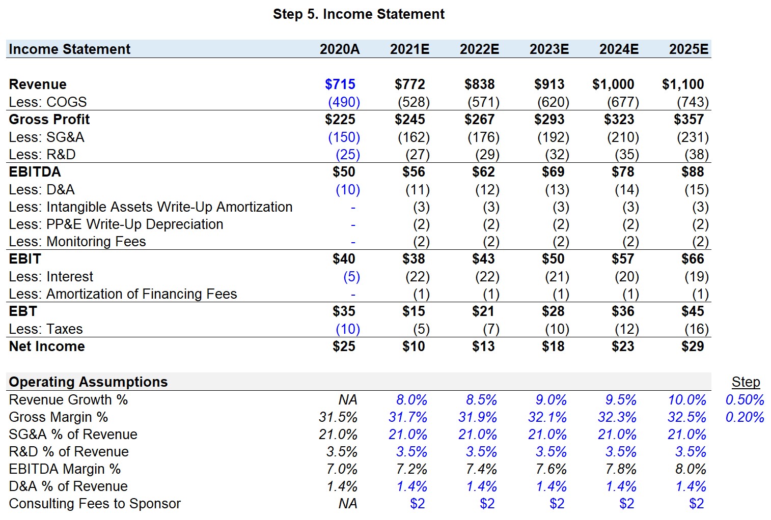
To start, we will first lay out the operating assumptions at the bottom and calculate the drivers based on revenue. For 2020A, we can see the gross margin is 31.5%, SG&A is 21.0% of revenue, R&D is 3.5% of revenue, and D&A is 1.4% of revenue.

Next, we will project revenue since most of the line items will be projected off revenue. As the prompt stated, the revenue growth rate in 2021 is 8%. Using a step function, we will increase this 8% by 0.5% each year. If done correctly, you should have 10.0% as the growth rate in 2025.

For the gross margin, we will again use a step function to increase it by 0.20% each year. In 2025, the gross margin should be 32.5%.

Then for SG&A, R&D, and D&A, we simply straight-line all of them for the forecast period.

I/S Forecast

With the operational assumptions laid out, we are now ready to forecast the income statement.

Starting with the top line, we will calculate revenue by multiplying the previous revenue amount by (1 + the YoY growth rate assumption).

For the gross profit, we will multiply the gross margin assumption by the current period revenue. To calculate COGS, we will back out of the amount by subtracting gross profit by revenue.

SG&A, R&D, and D&A will all be forecasted by multiplying the % assumption by revenue, just remember to include a negative sign in front since these all represent outflows of cash.

Next, below the D&A line item, we will account for the additional amortization and depreciation from the write-ups. The annual incremental amortization related to the intangible assets write-up is $3mm, while the incremental depreciation from the PP&E write-up is $1mm each year.

The last expense before the EBIT line item is the $2mm in monitoring fee paid to the private equity firm. This monitoring fee is an annual consulting fee paid by the portfolio company to the sponsor. Many private equity firms, particularly those that hire consultants, have many operating partners listed on their webpage, or is a subsidiary under a consulting firm (e.g. Bain Capital / Bain & Company), will arrange these types of advisory fees in their investment agreement to have an additional source of proceeds prior to the exit.

Just as a side note, monitoring fees are a controversial topic as the expense is tax-deductible for the portfolio companies and reduces the taxes paid. In many cases, however, no actual monitoring services are provided and the payments are instead “hidden dividends” paid to the private equity sponsor.

For interest, we will leave this section blank for now and return to it once the debt schedule has been completed.

The amortization of financing fees has been calculated as $8mm and will be amortized over 7 years. Thus, we will divide the $8mm by 7 to get roughly ~$1mm in amortization each year.

To calculate the taxes due, we will multiply the tax rate of 35% by EBT and after subtracting this amount from EBT we have arrived at net income.

Step 5: Formulas Used

• Revenue = Prior Revenue × (1 + Revenue Growth %)
• Gross Margin % = Gross Profit ÷ Revenue
• Gross Profit = Gross Margin % Assumption × Revenue
• Cost of Goods Sold (“COGS”) = Gross Profit – Revenue
• SG&A % of Revenue = SG&A ÷ Revenue
• SG&A = SG&A % of Revenue Assumption × Revenue
• R&D % of Revenue = R&D ÷ Revenue
• R&D = R&D % of Revenue × Revenue
• EBITDA = Gross Profit – SG&A – R&D
• EBITDA = Revenue × EBITDA Margin %
• D&A % of Revenue = D&A ÷ Revenue
• D&A = D&A % of Revenue Assumption × Revenue
• EBIT = EBITDA – D&A – Intangible Assets Write-Up Amortization – PP&E Write-Up Depreciation – Monitoring Fees
• Operating Margin = EBIT ÷ Revenue
• Amortization of Financing Fees = Total Financing Fees ÷ Financing Fees Amortization Period
• Taxes = Tax Rate % Assumption × EBT
• Net Income = EBT – Taxes
• Step Function: Previous Cell Amount + Fixed Step Amount

Step 6. Cash Flow Statement (CFS)

Next, we will forecast the cash flow statement. You may notice the free cash flow build we did in the Basic LBO modeling test is essentially just a mini-version of the cash flow statement.

Cash Flow from Operating Activities

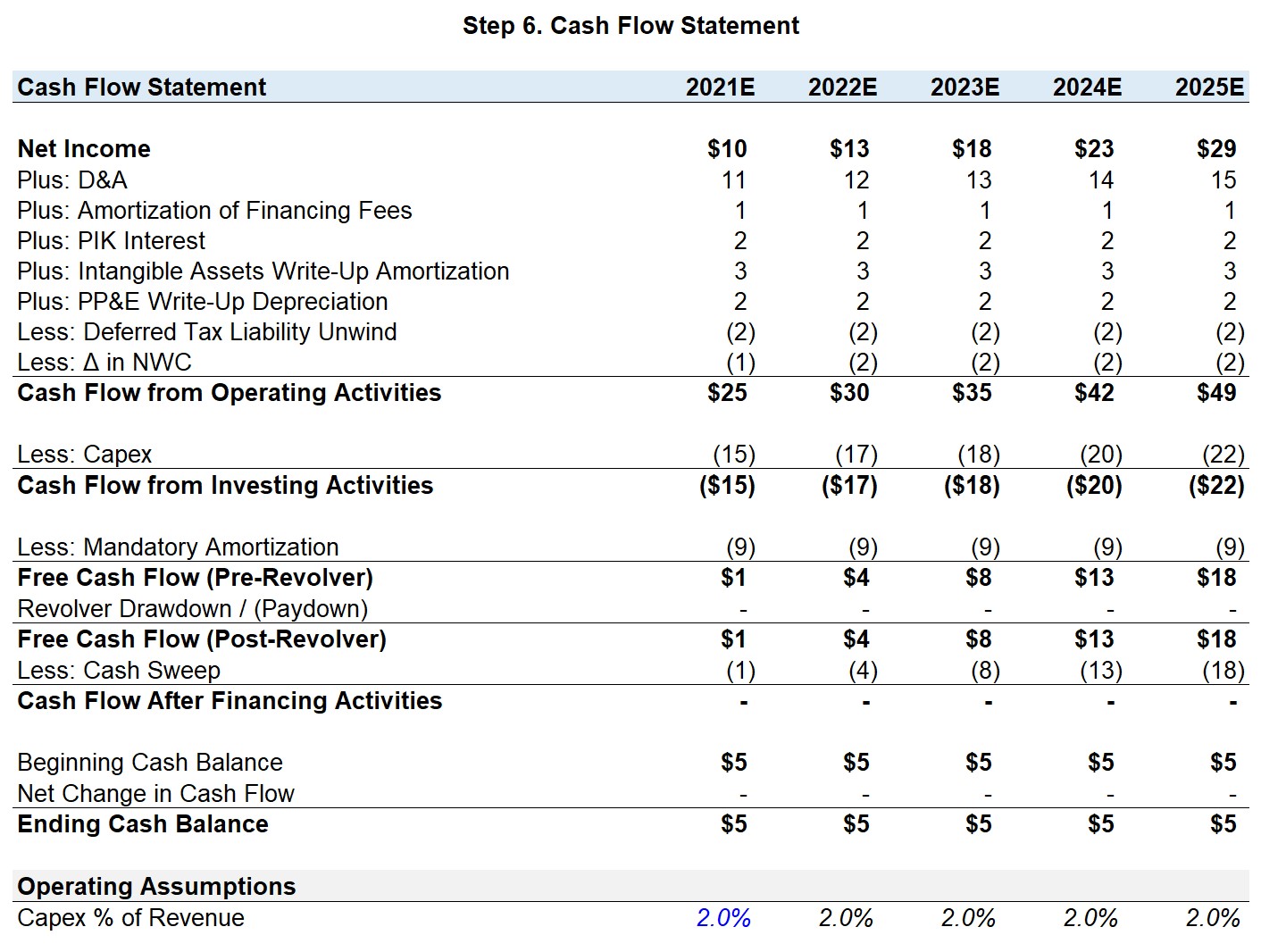
To begin filling out the cash flow statement, we will first grab net income from the income statement.

Next, we will adjust for the non-cash add-backs, which are D&A, Amortization of Financing Fees, PIK Interest, Intangible Assets Write-Up Amortization, and PP&E Write-Up Depreciation.

Except for PIK interest, we have all of the add-backs amounts calculated. Just make sure all the add-backs are shown as positives.

Next, we will subtract the annual deferred tax liability expense of $2mm and deduct the increase in NWC to arrive at cash flow from operating activities. Since we have not yet put the balance sheet together, the change in NWC will be left blank.

Cash Flow from Investing Activities

For the cash flow from investing activities section, the only line item is Capex, which will be 2% of revenue each year. Capex is the only line item directly forecasted on this CFS.

All that remains now is the Cash Flow from Financing section, which we will return to once the debt schedule has been completed.

Step 6 Formulas Used

• Cash Flow from Operating Activities = Net Income + D&A + Amortization of Financing Fees + PIK Interest + Intangible Assets Write-Up Amortization + PP&E Write-Up Depreciation – Deferred Tax Liability Unwind – Δ in NWC
• Deferred Tax Liability Unwind = Annual Unwind of DTL from Intangible Assets Write-Up + Annual Unwind of DTL from PP&E Write-Up
• Capex = Capex % of Revenue × Revenue
• Free Cash Flow (Pre-Revolver) = Cash Flow from Operating Activities – Cash Flow from Investing Activities – Mandatory Amortization
• Free Cash Flow (Post-Revolver) = Free Cash Flow Pre-Revolver – (Revolver Drawdown / Paydown)
• Cash Flow After Financing Activities = Free Cash Flow Post-Revolver – Cash Sweep
• Net Change in Cash Flow = Cash Flow After Financing Activities
• Ending Cash Balance = Beginning Cash Balance – Net Change in Cash

Step 7. Debt Schedule

When creating the debt schedule, we will go through each debt tranche in accordance with the waterfall logic (i.e. descending from highest seniority to lowest in the capital structure).

For all the debt tranches, we will utilize a roll-forward calculation.

Revolving Credit Facility (“Revolver”)

As mentioned in the prompt, the revolver was left undrawn during the initial purchase date.

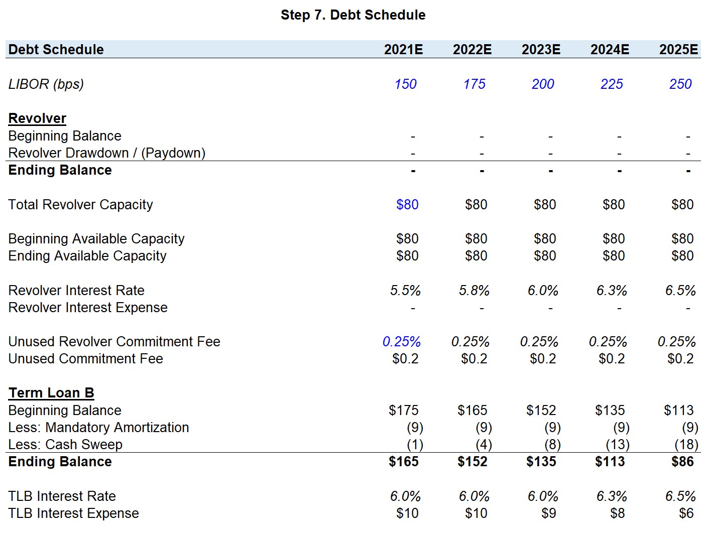
The “Total Revolver Capacity” was listed as 75% of the total LTM inventory and accounts receivable. If we sum up those two assets, we get $105mm, and multiplying it by 75% comes out to $79mm. To have a round number, we will add a “ROUND” function to the formula to get $80mm.

The maximum revolver capacity is generally based upon a borrowing-base lending formula (most often a certain percentage of A/R and inventory).

To get straight to the point, this revolving credit facility will be drawn from if the free cash flow (pre-revolver) dips below zero and a maximum of $80mm can be borrowed.

The pricing of the revolver was stated as LIBOR + 400, thus it is calculated as LIBOR + 4%. The LIBOR rates are listed at the top and are stated in terms of basis points (bps), as opposed to a percentage like the previous model test. Therefore, divide LIBOR by 10,000 in the formula.

Lastly, the unused revolver commitment fee is 0.25%, which is calculated by taking the average of the beginning and ending available revolver capacity and multiplying it by the fee %. If the revolver is left undrawn for the entire projection period, the unused commitment fee is $0.2mm each year.

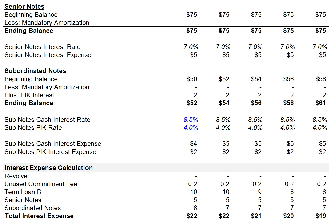
Term Loan B (“TLB”)

The next debt tranche is Term Loan B, in which $175mm was raised and this will be the beginning balance in 2021 of the roll-forward schedule.

The mandatory amortization was stated as 5%, so $9mm will be required to be paid out each year. To ensure there is no amortization once the principal has been paid down in full, we will include a “MIN” function with the mandatory amortization and the beginning TLB balance.

A new line item in the TLB roll-forward is the “Less: Cash Sweep”.

A cash sweep refers to the optional paydown of the principal when there is excess free cash flow remaining. The institutional lender of the TLB has given JoeCo the option to pay down more of the principal than the required 5%.

“Excess Free Cash Flow” is defined as the total cash balance minus the minimum cash balance required for normal business operations.

From the perspective of the lender, the principal of $175mm will be received by the end of maturity, and receiving it earlier is thus beneficial as the risk of not receiving the principal back (i.e. JoeCo underwent a bankruptcy) is decreased and the returned capital could be invested elsewhere.

But on the downside, the interest expense received by the lender decreases over time as more principal is paid down. As you can see from the interest expense calculation, the interest fell from $10mm in 2021 to $6mm by 2025.

The formula for the TLB cash sweep shown below utilizes a “-MIN” function between the beginning TLB balance after accounting for the mandatory amortization and the post-revolver FCF. If done correctly, the cash flow after financing activities should be zero in all the years.

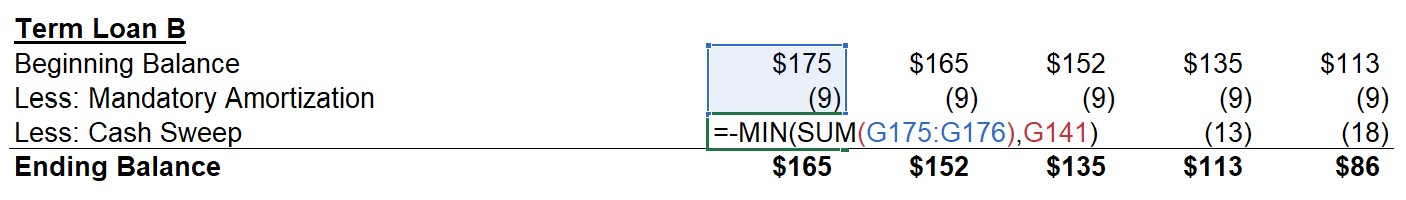
As we can see, all of the excess free cash flow is used to pay down as much debt as possible. The beginning balance of $175mm has decreased to $86mm by the end of 2025.

For the interest rate, the TLB is priced at LIBOR + 400 with a 2% floor. As you can see, for all the years when LIBOR is below 200 bps, the interest rate is 6%. But once LIBOR increases above 200 bps, the interest rate becomes 6.3% in 2024 and then 6.5% in 2025.

Senior Notes

The Senior Notes forecast is very straightforward. The beginning balance is $75mm and will remain unchanged throughout the entire holding period.

Given the fixed 7.0% interest rate, the interest expense will be $5mm each year.

Subordinated Notes

The final debt tranche is the subordinated notes, in which $50mm was raised.

As a reminder, the interest rate is 12.5% with 8.5% being paid-in-cash and a 4% PIK rate.

The cash interest is treated just like the interest on the senior notes. You simply take the average of the beginning and ending balance of the sub notes and multiply it by 8.5%.

As mentioned earlier, PIK interest is a non-cash payment that accrues over time.

While the cash interest portion is calculated based on the beginning and ending balance, the PIK will accrue based upon the beginning debt balance.

You can think of the PIK rate as the beginning Sub Note balance growing by 4% each year (i.e. multiply the beginning balance by 1.04 each year to see the next year’s beginning balance).

Notice how the initial balance is $50mm, but each year the ending balance increases. By 2025, the ending balance has grown to $61mm. Also, look at the side impact on the cash interest expense –because the beginning and ending balances have been growing, the cash interest expense increases too.

So, not only will the principal payment due at maturity be of a larger magnitude, the cash interest expense paid each year will be higher.

Interest Expense Calculation

To minimize the chance of making a linking error, it is useful to list out all the interest expenses when there were numerous debt tranches used.

While PIK is non-cash, it is included as part of the total interest expense calculation under accrual accounting. But then on the cash flow statement, the PIK interest will be added back to reflect it is not an actual cash outflow.

Recall that we skipped over the interest expense line item on the income statement, therefore we will link the ending interest expense balances to the relevant cells on the I/S.

Step 7: Formulas Used

• Total Revolver Capacity: “= ROUND ((Inventory + Accounts Receivable)*75%,-1)”
• Beginning Available Revolver Capacity = Total Revolver Capacity – Beginning Balance
• Ending Available Revolver Capacity = Beginning Available Capacity – (Revolver Drawdown / Paydown)
• Revolver Drawdown / (Paydown): “=MIN (Available Revolver Capacity, –MIN (Beginning Revolver Balance, Free Cash Flow Pre-Revolver)”
• Ending Revolver Balance = Beginning Revolver Balance + (Revolver Drawdown / Paydown)
• Revolver Interest Rate: “= MAX (LIBOR, Floor) + Spread”
• Revolver Interest Expense: “IF (Circularity Toggle = 1, AVERAGE (Beginning, Ending Revolver Balance), 0) × Revolver Interest Rate
• Revolver Unused Commitment Fee: “IF (Circularity Toggle = 1, AVERAGE (Beginning, Ending Available Revolver Capacity), 0) × Unused Commitment Fee %
• Term Loan B Mandatory Amortization: “= – MIN (TLB Raised * TLB Mandatory Amortization %, Beginning TLB Balance)”
• Term Loan B Cash Sweep: “– MIN (SUM(Beginning TLB Balance, Mandatory Amortization), Post-Revolver Free Cash Flow)”
• Ending Term Loan B Balance = Beginning TLB Balance – Mandatory TLB Amortization – Optional Cash Sweep
• Term Loan B Interest Rate: “= MAX (Floor, LIBOR / 10000) + (Spread / 10000)
• Term Loan B Interest Expense: “IF (Circularity Toggle = 1, AVERAGE (Beginning, Ending TLB Balance), 0) × TLB Interest Rate
• Senior Notes = Beginning Senior Notes Balance – Mandatory Amortization
• Senior Notes Interest Expense = “IF (Circularity Toggle = 1, AVERAGE (Beginning, Ending Senior Notes), 0) × Senior Notes Interest Rate
• Ending Balance Subordinated Notes = Beginning Balance Sub Notes – Mandatory Amortization + PIK Interest
• Sub Notes Cash Interest Expense: “IF (Circularity Toggle = 1, AVERAGE (Beginning, Ending Sub Notes), 0) × Sub Notes Cash Interest Rate
• Subordinated Notes PIK Interest Expense = Sub Notes PIK Rate × (Sub Notes Beginning Balance – Mandatory Amortization)
• Total Interest Expense = Revolver Interest + Unused Commitment Fee + TLB Interest + Senior Notes Interest + Subordinated Notes Interest

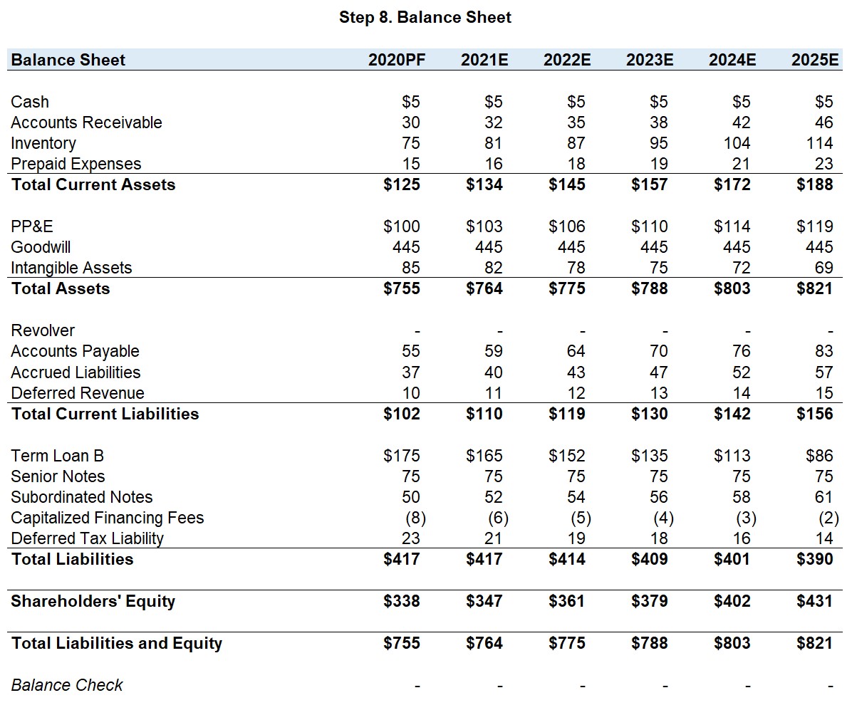
Step 8. Balance Sheet (B/S)

With the income statement and cash flow statement complete, we can fill out the balance sheet.

If you need a refresher on how to forecast the B/S items, read our Quick Reference Guide

Out of the three statements, the balance sheet should take the least amount of time to complete. Additionally, the B/S check will let you know if a mistake was made.

First, we will link to the PF B/S calculated earlier and bring it down to the 2020PF column. The reason we do this is to calculate the working capital % drivers and straight-line all of them, and because the non-working capital items all use the prior year balance in the formula (e.g. PP&E).

Assets Side

To start, cash will be pulled from the ending cash balance on the cash flow statement.

For the working capital assets, accounts receivable will be a function of Days Sales Outstanding (DSO), inventory will be based on Days Inventory Held (DIH), and prepaid expenses will be forecasted as a percentage of revenue.

Now moving onto the long-term assets, PP&E will be calculated as the prior balance plus Capex minus D&A and PP&E Write-Up Depreciation. Keep in mind, Capex will have been entered as a “-“, therefore subtract it in the Excel calculation to have the intended effect (i.e. Capex increases the PP&E balance)

For Goodwill, the $445mm balance will remain unchanged since there was no mention of impairments or Goodwill Amortization, which is an option available for private companies.

The final long-term asset, Intangible Assets, will be calculated as the prior balance minus the intangible assets write-up amortization. Notice the intangible assets balance decreases by ~$3mm each year.

Liabilities and Equity Side

Starting on the liabilities side, the revolver line item will be linked to the ending balance from the debt schedule.

The working capital liabilities such as accounts payable will be forecasted based on Days Payables Outstanding (DPO) and then accrued liabilities and deferred revenue will both be projected as a percentage of revenue.

For the long-term liabilities, the Term Loan B, Senior Notes, and Subordinated Notes will all be pulled from the ending balance from the debt schedule.

The capitalized financing fees will be shown as a negative $8mm in the PF year, and the Amortization of Financing Fees will be added to the balance each year.

The final liability, the deferred tax liability, will decrease by the change in DTLs calculated earlier.

Shareholders’ equity will be calculated as the prior balance plus net income since there were no dividends paid out.

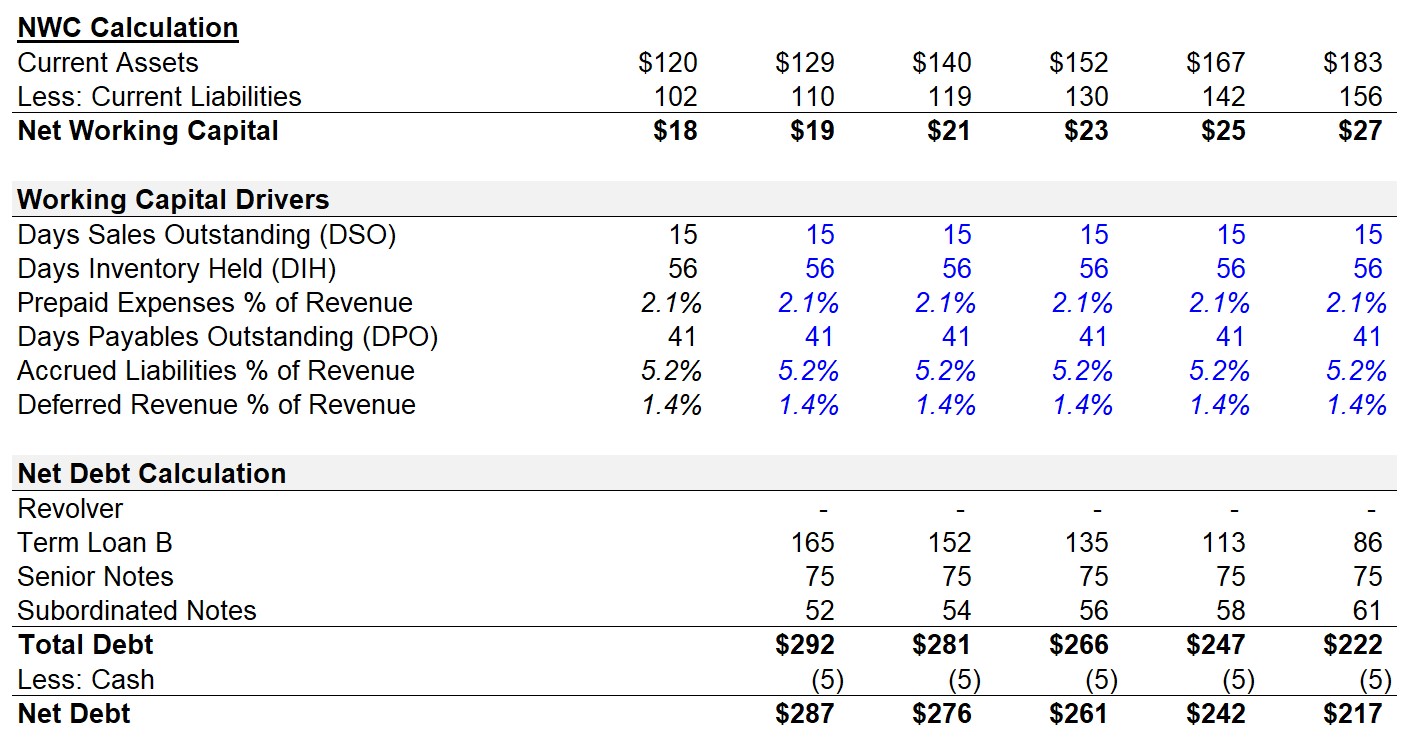
At this stage, the balance check will show the balance sheet is not in balance. The reason being, we skipped over the change in NWC on the CFS. Thus, we must calculate the NWC (Current Assets –Current Liabilities) and then link the YoY change (previous period NWC – current period NWC) on the cash flow statement.

Upon completion of this linkage, the balance sheet should now be in balance, or else a mistake was made somewhere.

Step 8: Formulas Used

• Days Sales Outstanding (DSO) = (Accounts Receivable ÷ Revenue) × 365
• Days Inventory Held (DIH) = (Inventory ÷ COGS) × 365
• Prepaid Expenses % of Revenue = Prepaid Expenses ÷ Revenue
• Days Payables Outstanding (DPO) = (Accounts Payable ÷ COGS) × 365
• Accrued Liabilities % of Revenue = Accrued Liabilities ÷ Revenue
• Deferred Revenue % of Revenue = Deferred Revenue ÷ Revenue
• Cash: Ending Cash Balance from Cash Roll-Forward on CFS
• Accounts Receivable = (DSO × Revenue) ÷ 365
• Inventory = (DIH × COGS) ÷ 365
• Prepaid Expenses = Prepaid Expenses % of Revenue × Revenue
• PP&E = Prior PP&E Balance + Capex – D&A – PP&E Write-Up Depreciation
• Intangible Assets = Prior Intangible Assets Balance – Intangible Assets Write-Up Amortization
• Accounts Payable = (DPO × COGS) ÷ 365
• Accrued Liabilities = Accrued Liabilities % of Revenue × Revenue
• Deferred Revenue = Deferred Revenue % of Revenue × Revenue
• All Debt Tranches (TLB, Senior Notes, Sub Notes): Ending Balance from Debt Schedule
• Capitalized Financing Fees = Prior Capitalized Financing Fees – Amortization of Financing Fees
• Deferred Tax Liability = Prior DTL – Deferred Tax Liability Unwind
• Net Working Capital = Current Assets – Current Liabilities
• Δ in NWC = Prior NWC – Current NWC
• Net Debt = Total Debt – Cash

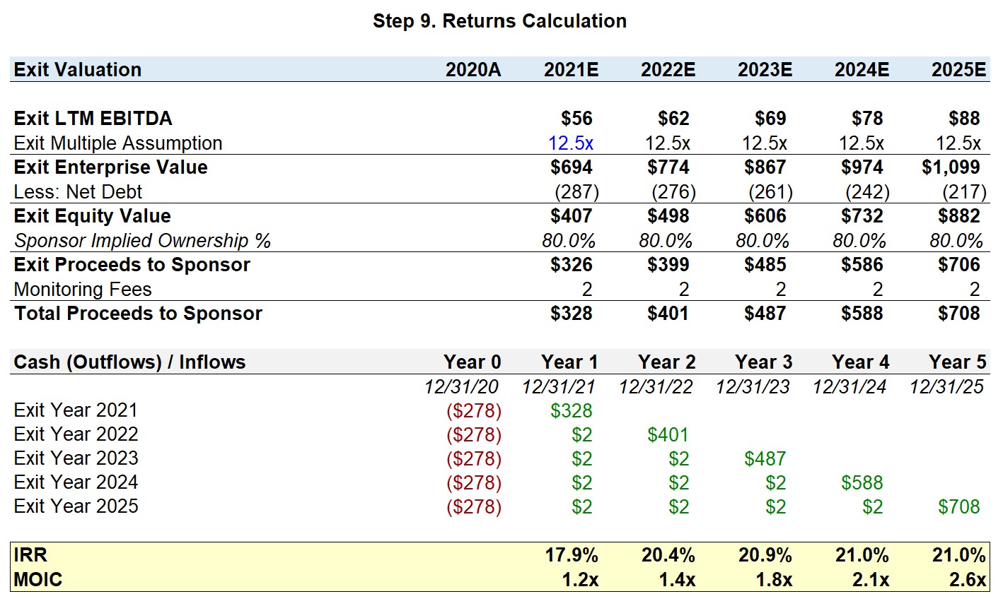
Step 9. Returns Calculation

We are now in the final steps of the modeling test, all that remains is calculating the returns metrics, creating the sensitivity tables, and answering the questions listed in the prompt.

Exit Valuation

To calculate the exit enterprise value, we multiply the exit multiple assumption by the exit LTM EBITDA. The conservative assumption is to assume the exit multiple is the same as the entry, thus we will use 12.5x as the exit multiple assumption.

Now, we will deduct the net debt to calculate the exit equity value.

This represents the total value of JoeCo to equity owners, but remember that management rolled over 20%. One minus the 20% rollover equity will give us the sponsor’s implied ownership, 80%.

Thereby, the “Exit Proceeds to Sponsor” will be calculated by multiplying the exit equity value by the 80% implied ownership.

But, recall that there is an additional source of proceeds for the PE firm, the annual monitoring fees. For this reason, we will link to the $2mm fee from the income statement each year (inflow).

The Cash (Outflows) / Inflows table should reflect both the exit proceeds and the monitoring fees. For example, for a five-year holding period – confirm that the PE firm received five $2mm payments in total.

With the Cash (Outflows) / Inflows table completed, we have the necessary cash flows to calculate the IRR and MOIC using Excel.

Step 9: Formulas Used

• Exit Enterprise Value = Exit Multiple × LTM EBITDA
• Exit Equity Value = Exit Enterprise Value – Net Debt
• Sponsor Implied Ownership % = 1 – Rollover Equity %
• Exit Proceeds to Sponsor = Exit Equity Value × Sponsor Implied Ownership %
• Total Proceeds to Sponsor = Exit Proceeds to Sponsor + Monitoring Fees
• IRR: “= XIRR (Range of Cash Flows, Range of Timing)”
• MOIC: “=SUM (Range of Inflows) / – Initial Outflow”

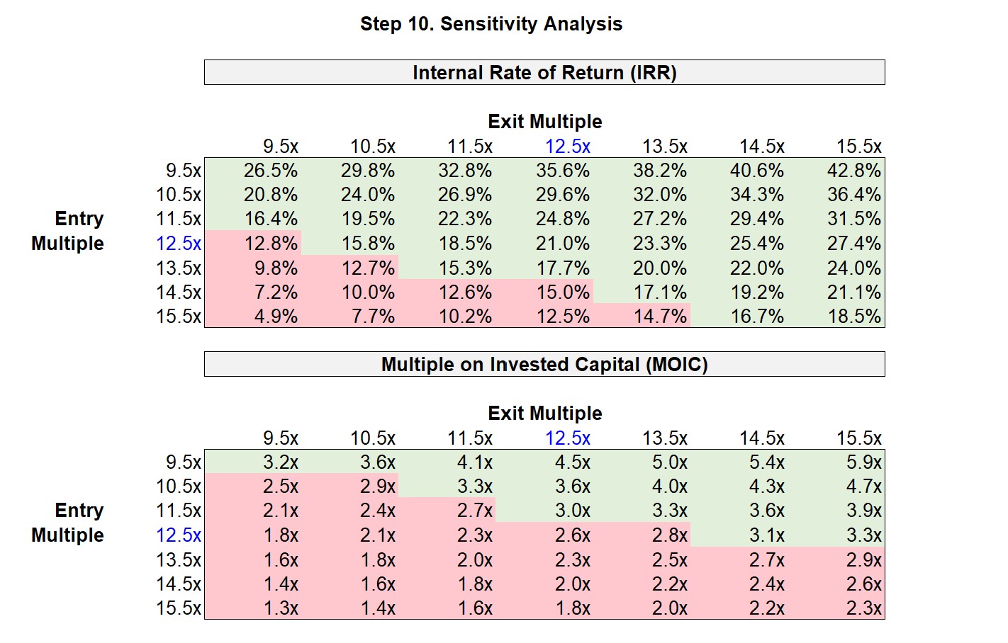
Step 10. Sensitivity Analysis

To create the sensitivity tables, first set the output variable in the top left corner – which will be either the IRR and MOIC for our purposes.

Highlight the table you have just set up and press “Alt + D + T”.

• The row input cell will be the exit multiple assumption in 2025 (Year 5)
• The column input will be the entry multiple assumption

To confirm you did the sensitivity table correctly, check to make sure that the highest value is on the top right, with the lowest being in the bottom left corner. The rationale being, a lower entry multiple and higher exit multiple yields the highest returns (and vice versa).

When answering the model test questions, the exact answers may not always be provided by the sensitivity tables (i.e. only approximations). But based on your best estimates, you can adjust the hardcoded input (blue font color) to find an exact figure you can reference in your answer.

For instance, we can estimate the lowest exit multiple to achieve an IRR of 15% seems to be between 9.5x and 10.5x from our sensitivity table. After a handful of iterations we can figure out that when the exit multiple input is 10.22x, the IRR is exactly 15.0%.

Standard LBO Modeling Test Conclusion

To conclude this article, we will answer the three questions listed in the prompt.

1. Assuming the private equity firm exits at the same multiple as entry after a five-year horizon, the IRR would be 21.0% and the MOIC would be 2.6x
2. To achieve a 3.0x MOIC in five years, the private equity firm would have to sell at a 14.0x exit multiple.
3. If the minimum IRR threshold is 15.0%, the lowest exit multiple that the private equity firm could exit at is approximately 10.3x.

Master LBO Modeling Our Advanced LBO Modeling course will teach you how to build a comprehensive LBO model and give you the confidence to ace the finance interview.

Learn More